Karina Bartolome: Pipelines en Scikit-Learn

Karina Bartolomé

Introducción

scikit-learn¹ 📦 es uno de los paquetes más utilizados para ajustar modelos de aprendizaje automático (machine learning). En este post, se presentan algunas alternativas de modelado mediante el uso de pipelines. El objetivo del posteo es introducir diversas técnicas implementadas en sklearn. No se busca mejorar la performance de un modelo, solo ilustrar posibles alternativas.

EN PROCESO

Conda environment 🐍

⚙️ Se utiliza un environment específico para este proyecto, con python 3.10:

reticulate::conda_create(envname='scikit-learn', python_version="3.10")

Se instalan los paquetes python 📦

reticulate::conda_install(envname='scikit-learn', 
                          packages='numpy', channel = 'conda-forge')

reticulate::conda_install(envname='scikit-learn', 
                          packages='pandas', channel = 'conda-forge')

reticulate::conda_install(envname='scikit-learn', 
                          packages='scikit-learn=1.1.1', channel = 'conda-forge')

reticulate::conda_install(envname = 'scikit-learn',
                          packages = 'scikit-optimize', channel='conda-forge')

reticulate::conda_install(envname = 'scikit-learn', 
                          packages='lightgbm', channel='conda-forge')

reticulate::conda_install(envname = 'scikit-learn', 
                          packages='jinja2', channel='conda-forge')

Con el environment creado y activado, se define que se va a utilizar ese environment:

reticulate::use_condaenv(condaenv = 'scikit-learn', required = TRUE)

Para utilizar python en rmarkdown, es necesario definir que se va a utilizar un chunk de código python. Para más información sobre python en rmarkdown, ver: El uso de múltiples lenguajes en Rmarkdown.

Librerías 📚

Para realizar algunos gráficos y tablas se utilizará R y los pipelines de modelado se utilizará python. A continuación se cargan las librerías a utilizar.

🔹 Las librerías de R se cargan utilizando un chunk R:

Show code

library(reticulate)
library(tidyverse)
library(tidymodels)
library(gt)
library(sknifedatar)

🔹Se utiliza un chunk python para cargar las librerías de python:

Show code

import pandas as pd
import numpy as np
from scipy.stats import randint as sp_randInt
import scipy.stats as st

# Viz
import matplotlib.pyplot as plt
import seaborn as sns
cm = sns.color_palette("ch:start=.2,rot=-.3", as_cmap=True)

# Partición en train y test
from sklearn.model_selection import train_test_split

# Pipelines
from sklearn.pipeline import Pipeline, FeatureUnion
from sklearn.compose import ColumnTransformer, make_column_selector
from sklearn.compose import TransformedTargetRegressor
from sklearn.base import BaseEstimator, TransformerMixin

# Preprocesamiento
from sklearn.impute import SimpleImputer
from sklearn.preprocessing import OneHotEncoder
from sklearn.preprocessing import StandardScaler
from sklearn.preprocessing import RobustScaler
from sklearn.decomposition import PCA

# Selección de variables
from sklearn.feature_selection import (
  SelectKBest,
  VarianceThreshold,
  r_regression,
  f_regression,
  mutual_info_regression)

# Modelos
from sklearn.linear_model import LinearRegression
from sklearn.ensemble import RandomForestRegressor
from lightgbm import LGBMRegressor
from sklearn.model_selection import cross_validate

# Métricas
from sklearn import metrics

# Optimización
from sklearn.model_selection import RandomizedSearchCV, GridSearchCV
from skopt import BayesSearchCV
from skopt.space import Real, Categorical, Integer
from skopt.plots import plot_objective, plot_histogram

Show code

pd.set_option('display.max_columns', 20)
pd.options.display.float_format = "{:,.2f}".format
import warnings
warnings.filterwarnings(action='ignore', category=UserWarning, module='sklearn')

ITERS = 50
CV_FOLDS = 5
METRICA = 'neg_root_mean_squared_error'

1. Datos 📊

Se utilizan datos de Kaggle, con el objetivo de aplicar modelos de regresión para estimar precios de propiedades a partir de un conjunto de variables provisto.

kaggle competitions download -c house-prices-advanced-regression-techniques

Show code

df_train = pd.read_csv('data/train.csv')
df_test = pd.read_csv('data/test.csv')

print('En total hay',df_train.shape[0],'observaciones')

En total hay 1460 observaciones

Show code

(df_train.describe().T
  .style
  .background_gradient(
    subset=['min', '25%', '50%', '75%', 'max'], 
    axis=1, 
    cmap=cm)
  .format(precision=3)
)

	count	mean	std	min	25%	50%	75%	max
Id	1460.000	730.500	421.610	1.000	365.750	730.500	1095.250	1460.000
MSSubClass	1460.000	56.897	42.301	20.000	20.000	50.000	70.000	190.000
LotFrontage	1201.000	70.050	24.285	21.000	59.000	69.000	80.000	313.000
LotArea	1460.000	10516.828	9981.265	1300.000	7553.500	9478.500	11601.500	215245.000
OverallQual	1460.000	6.099	1.383	1.000	5.000	6.000	7.000	10.000
OverallCond	1460.000	5.575	1.113	1.000	5.000	5.000	6.000	9.000
YearBuilt	1460.000	1971.268	30.203	1872.000	1954.000	1973.000	2000.000	2010.000
YearRemodAdd	1460.000	1984.866	20.645	1950.000	1967.000	1994.000	2004.000	2010.000
MasVnrArea	1452.000	103.685	181.066	0.000	0.000	0.000	166.000	1600.000
BsmtFinSF1	1460.000	443.640	456.098	0.000	0.000	383.500	712.250	5644.000
BsmtFinSF2	1460.000	46.549	161.319	0.000	0.000	0.000	0.000	1474.000
BsmtUnfSF	1460.000	567.240	441.867	0.000	223.000	477.500	808.000	2336.000
TotalBsmtSF	1460.000	1057.429	438.705	0.000	795.750	991.500	1298.250	6110.000
1stFlrSF	1460.000	1162.627	386.588	334.000	882.000	1087.000	1391.250	4692.000
2ndFlrSF	1460.000	346.992	436.528	0.000	0.000	0.000	728.000	2065.000
LowQualFinSF	1460.000	5.845	48.623	0.000	0.000	0.000	0.000	572.000
GrLivArea	1460.000	1515.464	525.480	334.000	1129.500	1464.000	1776.750	5642.000
BsmtFullBath	1460.000	0.425	0.519	0.000	0.000	0.000	1.000	3.000
BsmtHalfBath	1460.000	0.058	0.239	0.000	0.000	0.000	0.000	2.000
FullBath	1460.000	1.565	0.551	0.000	1.000	2.000	2.000	3.000
HalfBath	1460.000	0.383	0.503	0.000	0.000	0.000	1.000	2.000
BedroomAbvGr	1460.000	2.866	0.816	0.000	2.000	3.000	3.000	8.000
KitchenAbvGr	1460.000	1.047	0.220	0.000	1.000	1.000	1.000	3.000
TotRmsAbvGrd	1460.000	6.518	1.625	2.000	5.000	6.000	7.000	14.000
Fireplaces	1460.000	0.613	0.645	0.000	0.000	1.000	1.000	3.000
GarageYrBlt	1379.000	1978.506	24.690	1900.000	1961.000	1980.000	2002.000	2010.000
GarageCars	1460.000	1.767	0.747	0.000	1.000	2.000	2.000	4.000
GarageArea	1460.000	472.980	213.805	0.000	334.500	480.000	576.000	1418.000
WoodDeckSF	1460.000	94.245	125.339	0.000	0.000	0.000	168.000	857.000
OpenPorchSF	1460.000	46.660	66.256	0.000	0.000	25.000	68.000	547.000
EnclosedPorch	1460.000	21.954	61.119	0.000	0.000	0.000	0.000	552.000
3SsnPorch	1460.000	3.410	29.317	0.000	0.000	0.000	0.000	508.000
ScreenPorch	1460.000	15.061	55.757	0.000	0.000	0.000	0.000	480.000
PoolArea	1460.000	2.759	40.177	0.000	0.000	0.000	0.000	738.000
MiscVal	1460.000	43.489	496.123	0.000	0.000	0.000	0.000	15500.000
MoSold	1460.000	6.322	2.704	1.000	5.000	6.000	8.000	12.000
YrSold	1460.000	2007.816	1.328	2006.000	2007.000	2008.000	2009.000	2010.000
SalePrice	1460.000	180921.196	79442.503	34900.000	129975.000	163000.000	214000.000	755000.000

Se eliminan las variables con demasiados valores faltantes:

cols_to_drop = df_train.columns[df_train.isna().mean() >= 0.5]
vars = [x for x in df_train.columns if x not in cols_to_drop]

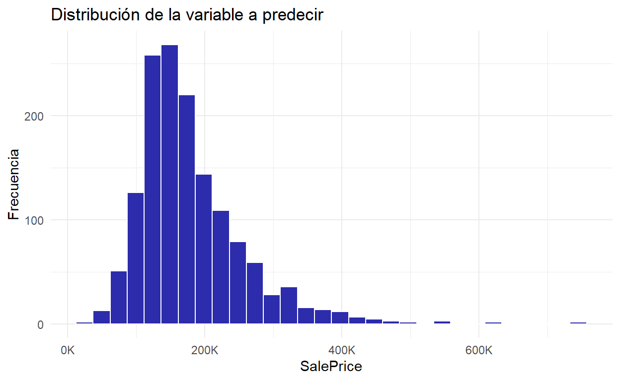
df_train = df_train[vars]

Se visualiza la distribución de la variable a predecir:

Show code

py$df_train %>%
  ggplot(aes(x = SalePrice)) +
  geom_histogram() +
  scale_x_continuous(
    labels = scales::label_number(scale = 1 / 1000, suffix = 'K')) +
  geom_histogram(color = 'white',  fill = colores[1],  alpha = 0.5) +
  labs(
    x = 'SalePrice',
    y = 'Frecuencia',
    title = 'Distribución de la variable a predecir'
  )

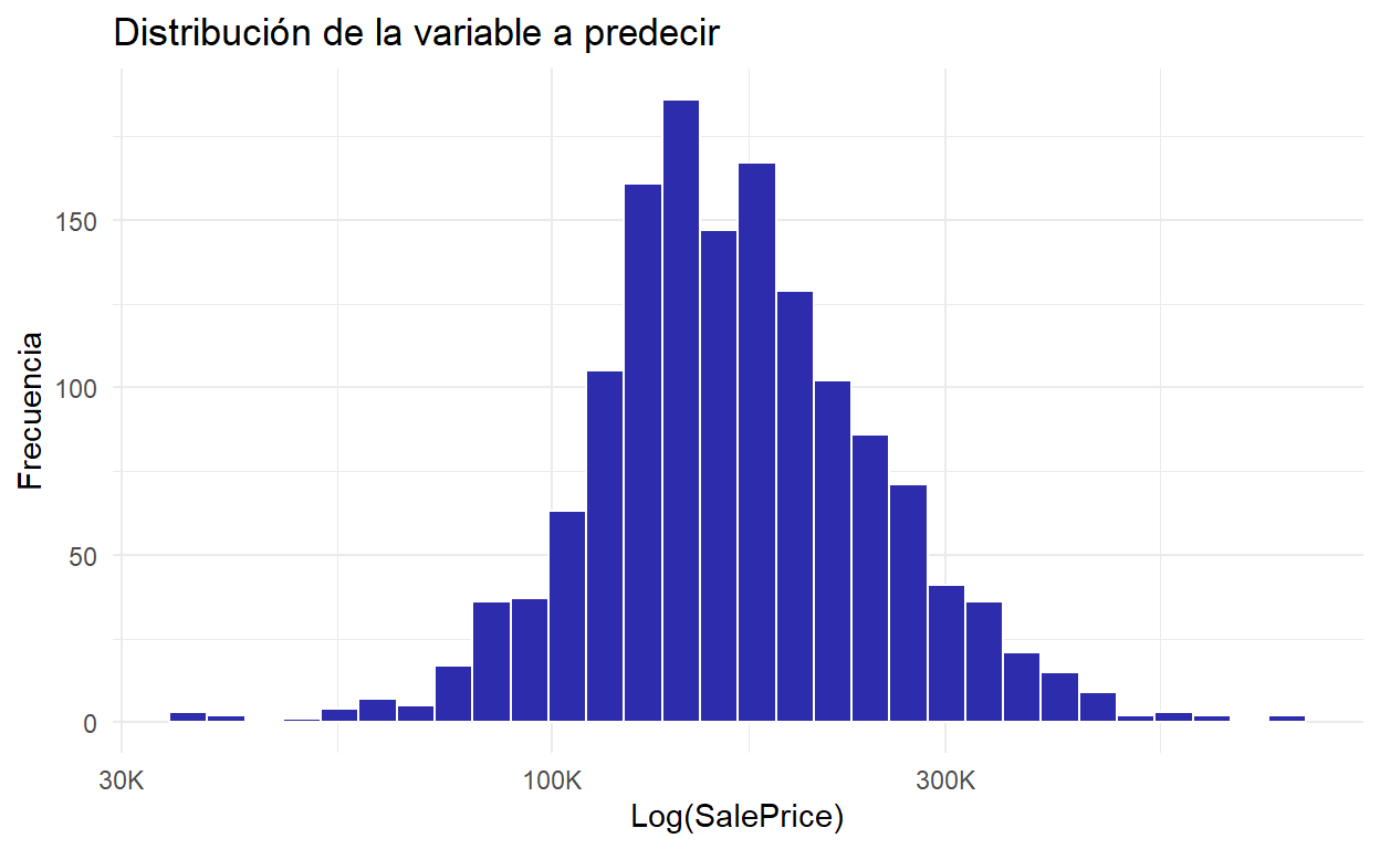
En escala Log:

Show code

py$df_train %>%
  ggplot(aes(x = SalePrice)) +
  geom_histogram() +
  scale_x_log10(
    labels = scales::label_number(scale = 1 / 1000, suffix = 'K')) +
  geom_histogram(color = 'white',  fill = colores[1],  alpha = 0.5) +
  labs(
    x = 'Log(SalePrice)',
    y = 'Frecuencia',
    title = 'Distribución de la variable a predecir'
  )

2. Partición en train y test ✂️

y = np.array(df_train['SalePrice'])
X = df_train.drop(['Id','SalePrice'], axis=1)

X_train, X_test, y_train, y_test = train_test_split(
    X, y,
    test_size    = 0.25, 
    random_state = 42, 
)

print('Cantidad de observaciones en train:', X_train.shape[0])

Cantidad de observaciones en train: 1095

print('Cantidad de observaciones en test:', X_test.shape[0])

Cantidad de observaciones en test: 365

print('En train el precio promedio es $', round(y_train.mean(),2))

En train el precio promedio es $ 181712.29

print('En test el precio promedio es $', round(y_test.mean(),2))

En test el precio promedio es $ 178547.92

3. Pipeline de preprocesamiento ⚙️

vars_categoricas = list(X.select_dtypes(include=['object']).columns)
vars_numericas   = list(X.select_dtypes(exclude=['object']).columns)

preprocess_modeimpute = SimpleImputer(
  missing_values=np.nan, strategy='most_frequent')
preprocess_meanimpute = SimpleImputer(
  missing_values=np.nan, strategy="median")
preprocess_onehot = OneHotEncoder(
  handle_unknown="infrequent_if_exist", 
  min_frequency = 0.1, drop='if_binary')
preprocess_scaler = StandardScaler()
preprocess_nzv = VarianceThreshold(
  threshold=0.05)


# Preprocesador para variables categóricas
categorical_preprocessor = Pipeline([
  ('mode_impute', preprocess_modeimpute),
  ('one-hot-encoding', preprocess_onehot),
])

# Preprocesador para variables numéricas
numerical_preprocessor = Pipeline([
  ('nzv', preprocess_nzv),
  ("imputation_mean", preprocess_meanimpute),
  ('scaler', preprocess_scaler),
])


# Preprocesador completo
preprocessor = Pipeline([
        ('Preprocesamiento inicial', ColumnTransformer([
          ('numericas', numerical_preprocessor, vars_numericas),
          ('categoricas', categorical_preprocessor, vars_categoricas),
          ], remainder='drop')
        ),
])

Se ajusta el pipeline para preprocesamiento:

preprocessor.fit(X_train)

Pipeline(steps=[('Preprocesamiento inicial',
                 ColumnTransformer(transformers=[('numericas',
                                                  Pipeline(steps=[('nzv',
                                                                   VarianceThreshold(threshold=0.05)),
                                                                  ('imputation_mean',
                                                                   SimpleImputer(strategy='median')),
                                                                  ('scaler',
                                                                   StandardScaler())]),
                                                  ['MSSubClass', 'LotFrontage',
                                                   'LotArea', 'OverallQual',
                                                   'OverallCond', 'YearBuilt',
                                                   'YearRemodAdd', 'MasVnrArea',
                                                   'BsmtFinSF1', 'B...
                                                   'LotShape', 'LandContour',
                                                   'Utilities', 'LotConfig',
                                                   'LandSlope', 'Neighborhood',
                                                   'Condition1', 'Condition2',
                                                   'BldgType', 'HouseStyle',
                                                   'RoofStyle', 'RoofMatl',
                                                   'Exterior1st', 'Exterior2nd',
                                                   'MasVnrType', 'ExterQual',
                                                   'ExterCond', 'Foundation',
                                                   'BsmtQual', 'BsmtCond',
                                                   'BsmtExposure',
                                                   'BsmtFinType1',
                                                   'BsmtFinType2', 'Heating',
                                                   'HeatingQC', 'CentralAir',
                                                   'Electrical', 'KitchenQual', ...])]))])

In a Jupyter environment, please rerun this cell to show the HTML representation or trust the notebook.
On GitHub, the HTML representation is unable to render, please try loading this page with nbviewer.org.

Pipeline

Pipeline(steps=[('Preprocesamiento inicial',
                 ColumnTransformer(transformers=[('numericas',
                                                  Pipeline(steps=[('nzv',
                                                                   VarianceThreshold(threshold=0.05)),
                                                                  ('imputation_mean',
                                                                   SimpleImputer(strategy='median')),
                                                                  ('scaler',
                                                                   StandardScaler())]),
                                                  ['MSSubClass', 'LotFrontage',
                                                   'LotArea', 'OverallQual',
                                                   'OverallCond', 'YearBuilt',
                                                   'YearRemodAdd', 'MasVnrArea',
                                                   'BsmtFinSF1', 'B...
                                                   'LotShape', 'LandContour',
                                                   'Utilities', 'LotConfig',
                                                   'LandSlope', 'Neighborhood',
                                                   'Condition1', 'Condition2',
                                                   'BldgType', 'HouseStyle',
                                                   'RoofStyle', 'RoofMatl',
                                                   'Exterior1st', 'Exterior2nd',
                                                   'MasVnrType', 'ExterQual',
                                                   'ExterCond', 'Foundation',
                                                   'BsmtQual', 'BsmtCond',
                                                   'BsmtExposure',
                                                   'BsmtFinType1',
                                                   'BsmtFinType2', 'Heating',
                                                   'HeatingQC', 'CentralAir',
                                                   'Electrical', 'KitchenQual', ...])]))])

Preprocesamiento inicial: ColumnTransformer

ColumnTransformer(transformers=[('numericas',
                                 Pipeline(steps=[('nzv',
                                                  VarianceThreshold(threshold=0.05)),
                                                 ('imputation_mean',
                                                  SimpleImputer(strategy='median')),
                                                 ('scaler', StandardScaler())]),
                                 ['MSSubClass', 'LotFrontage', 'LotArea',
                                  'OverallQual', 'OverallCond', 'YearBuilt',
                                  'YearRemodAdd', 'MasVnrArea', 'BsmtFinSF1',
                                  'BsmtFinSF2', 'BsmtUnfSF', 'TotalBsmtSF',
                                  '1stFl...
                                  'LandContour', 'Utilities', 'LotConfig',
                                  'LandSlope', 'Neighborhood', 'Condition1',
                                  'Condition2', 'BldgType', 'HouseStyle',
                                  'RoofStyle', 'RoofMatl', 'Exterior1st',
                                  'Exterior2nd', 'MasVnrType', 'ExterQual',
                                  'ExterCond', 'Foundation', 'BsmtQual',
                                  'BsmtCond', 'BsmtExposure', 'BsmtFinType1',
                                  'BsmtFinType2', 'Heating', 'HeatingQC',
                                  'CentralAir', 'Electrical', 'KitchenQual', ...])])

numericas

['MSSubClass', 'LotFrontage', 'LotArea', 'OverallQual', 'OverallCond', 'YearBuilt', 'YearRemodAdd', 'MasVnrArea', 'BsmtFinSF1', 'BsmtFinSF2', 'BsmtUnfSF', 'TotalBsmtSF', '1stFlrSF', '2ndFlrSF', 'LowQualFinSF', 'GrLivArea', 'BsmtFullBath', 'BsmtHalfBath', 'FullBath', 'HalfBath', 'BedroomAbvGr', 'KitchenAbvGr', 'TotRmsAbvGrd', 'Fireplaces', 'GarageYrBlt', 'GarageCars', 'GarageArea', 'WoodDeckSF', 'OpenPorchSF', 'EnclosedPorch', '3SsnPorch', 'ScreenPorch', 'PoolArea', 'MiscVal', 'MoSold', 'YrSold']

VarianceThreshold

VarianceThreshold(threshold=0.05)

SimpleImputer

SimpleImputer(strategy='median')

StandardScaler

StandardScaler()

categoricas

['MSZoning', 'Street', 'LotShape', 'LandContour', 'Utilities', 'LotConfig', 'LandSlope', 'Neighborhood', 'Condition1', 'Condition2', 'BldgType', 'HouseStyle', 'RoofStyle', 'RoofMatl', 'Exterior1st', 'Exterior2nd', 'MasVnrType', 'ExterQual', 'ExterCond', 'Foundation', 'BsmtQual', 'BsmtCond', 'BsmtExposure', 'BsmtFinType1', 'BsmtFinType2', 'Heating', 'HeatingQC', 'CentralAir', 'Electrical', 'KitchenQual', 'Functional', 'FireplaceQu', 'GarageType', 'GarageFinish', 'GarageQual', 'GarageCond', 'PavedDrive', 'SaleType', 'SaleCondition']

SimpleImputer

SimpleImputer(strategy='most_frequent')

OneHotEncoder

OneHotEncoder(drop='if_binary', handle_unknown='infrequent_if_exist',
              min_frequency=0.1)

Se transforma el dataframe original con el pipeline generado:

X_processed = pd.DataFrame(
  preprocessor.transform(X_train), 
  columns = preprocessor.get_feature_names_out()
)

Notar que al visualizar las primeras dos observaciones luego del pipeline de preprocesamiento anterior se cuenta con una gran cantidad de variables:

py$X_processed %>% 
  head(2) %>% 
  gt() %>% 
  tab_header(
    title=md('**Datos post preprocesamiento**: variables para modelado'),
    subtitle = 'Los nombres de las variables contienen el prefijo del nombre del 
      pipeline de preprocesamiento, en este caso: numéricas o categóricas'
  ) %>% 
  opt_align_table_header(align='left') %>% 
  fmt_number(everything(), decimals=2)

numericas__MSSubClass	numericas__LotFrontage	numericas__LotArea	numericas__OverallQual	numericas__OverallCond	numericas__YearBuilt	numericas__YearRemodAdd	numericas__MasVnrArea	numericas__BsmtFinSF1	numericas__BsmtFinSF2	numericas__BsmtUnfSF	numericas__TotalBsmtSF	numericas__1stFlrSF	numericas__2ndFlrSF	numericas__LowQualFinSF	numericas__GrLivArea	numericas__BsmtFullBath	numericas__BsmtHalfBath	numericas__FullBath	numericas__HalfBath	numericas__BedroomAbvGr	numericas__TotRmsAbvGrd	numericas__Fireplaces	numericas__GarageYrBlt	numericas__GarageCars	numericas__GarageArea	numericas__WoodDeckSF	numericas__OpenPorchSF	numericas__EnclosedPorch	numericas__3SsnPorch	numericas__ScreenPorch	numericas__PoolArea	numericas__MiscVal	numericas__MoSold	numericas__YrSold	categoricas__MSZoning_RL	categoricas__MSZoning_RM	categoricas__MSZoning_infrequent_sklearn	categoricas__Street_infrequent_sklearn	categoricas__LotShape_IR1	categoricas__LotShape_Reg	categoricas__LotShape_infrequent_sklearn	categoricas__LandContour_infrequent_sklearn	categoricas__Utilities_infrequent_sklearn	categoricas__LotConfig_Corner	categoricas__LotConfig_Inside	categoricas__LotConfig_infrequent_sklearn	categoricas__LandSlope_infrequent_sklearn	categoricas__Neighborhood_CollgCr	categoricas__Neighborhood_NAmes	categoricas__Neighborhood_infrequent_sklearn	categoricas__Condition1_infrequent_sklearn	categoricas__Condition2_infrequent_sklearn	categoricas__BldgType_infrequent_sklearn	categoricas__HouseStyle_1.5Fin	categoricas__HouseStyle_1Story	categoricas__HouseStyle_2Story	categoricas__HouseStyle_infrequent_sklearn	categoricas__RoofStyle_Gable	categoricas__RoofStyle_Hip	categoricas__RoofStyle_infrequent_sklearn	categoricas__RoofMatl_infrequent_sklearn	categoricas__Exterior1st_HdBoard	categoricas__Exterior1st_MetalSd	categoricas__Exterior1st_VinylSd	categoricas__Exterior1st_Wd Sdng	categoricas__Exterior1st_infrequent_sklearn	categoricas__Exterior2nd_HdBoard	categoricas__Exterior2nd_MetalSd	categoricas__Exterior2nd_VinylSd	categoricas__Exterior2nd_Wd Sdng	categoricas__Exterior2nd_infrequent_sklearn	categoricas__MasVnrType_BrkFace	categoricas__MasVnrType_None	categoricas__MasVnrType_infrequent_sklearn	categoricas__ExterQual_Gd	categoricas__ExterQual_TA	categoricas__ExterQual_infrequent_sklearn	categoricas__ExterCond_infrequent_sklearn	categoricas__Foundation_CBlock	categoricas__Foundation_PConc	categoricas__Foundation_infrequent_sklearn	categoricas__BsmtQual_Gd	categoricas__BsmtQual_TA	categoricas__BsmtQual_infrequent_sklearn	categoricas__BsmtCond_infrequent_sklearn	categoricas__BsmtExposure_Av	categoricas__BsmtExposure_No	categoricas__BsmtExposure_infrequent_sklearn	categoricas__BsmtFinType1_ALQ	categoricas__BsmtFinType1_BLQ	categoricas__BsmtFinType1_GLQ	categoricas__BsmtFinType1_Unf	categoricas__BsmtFinType1_infrequent_sklearn	categoricas__BsmtFinType2_infrequent_sklearn	categoricas__Heating_infrequent_sklearn	categoricas__HeatingQC_Ex	categoricas__HeatingQC_Gd	categoricas__HeatingQC_TA	categoricas__HeatingQC_infrequent_sklearn	categoricas__CentralAir_infrequent_sklearn	categoricas__Electrical_infrequent_sklearn	categoricas__KitchenQual_Gd	categoricas__KitchenQual_TA	categoricas__KitchenQual_infrequent_sklearn	categoricas__Functional_infrequent_sklearn	categoricas__FireplaceQu_Gd	categoricas__FireplaceQu_TA	categoricas__FireplaceQu_infrequent_sklearn	categoricas__GarageType_Attchd	categoricas__GarageType_Detchd	categoricas__GarageType_infrequent_sklearn	categoricas__GarageFinish_Fin	categoricas__GarageFinish_RFn	categoricas__GarageFinish_Unf	categoricas__GarageQual_infrequent_sklearn	categoricas__GarageCond_infrequent_sklearn	categoricas__PavedDrive_infrequent_sklearn	categoricas__SaleType_infrequent_sklearn	categoricas__SaleCondition_infrequent_sklearn
Datos post preprocesamiento: variables para modelado
Los nombres de las variables contienen el prefijo del nombre del pipeline de preprocesamiento, en este caso: numéricas o categóricas
1.48	−1.20	−0.68	0.64	−0.52	1.11	1.02	−0.52	−0.94	−0.28	1.71	0.64	0.86	−0.81	−0.12	−0.05	−0.81	−0.24	0.77	−0.77	−1.11	0.27	0.59	1.09	0.29	−0.19	0.46	−0.43	−0.34	−0.12	−0.28	−0.07	−0.12	−0.51	0.14	1.00	0.00	0.00	0.00	0.00	1.00	0.00	0.00	0.00	0.00	1.00	0.00	0.00	0.00	0.00	1.00	0.00	0.00	1.00	0.00	1.00	0.00	0.00	1.00	0.00	0.00	0.00	0.00	0.00	1.00	0.00	0.00	0.00	0.00	1.00	0.00	0.00	1.00	0.00	0.00	1.00	0.00	0.00	0.00	0.00	1.00	0.00	1.00	0.00	0.00	1.00	0.00	1.00	0.00	0.00	0.00	1.00	0.00	0.00	0.00	0.00	1.00	0.00	0.00	0.00	0.00	0.00	1.00	0.00	0.00	0.00	1.00	0.00	0.00	1.00	0.00	0.00	1.00	0.00	0.00	0.00	0.00	0.00	0.00	0.00
−0.87	0.34	−0.05	−0.09	0.39	0.09	0.68	−0.02	0.47	2.17	−1.28	−0.05	0.36	−0.81	−0.12	−0.42	1.12	−0.24	−1.06	1.25	0.13	−0.96	0.59	−0.20	0.29	0.03	1.30	−0.72	−0.34	−0.12	−0.28	15.00	−0.12	−2.00	−1.37	1.00	0.00	0.00	0.00	0.00	1.00	0.00	0.00	0.00	0.00	1.00	0.00	0.00	0.00	0.00	1.00	0.00	0.00	0.00	0.00	1.00	0.00	0.00	0.00	1.00	0.00	0.00	1.00	0.00	0.00	0.00	0.00	1.00	0.00	0.00	0.00	0.00	1.00	0.00	0.00	0.00	1.00	0.00	0.00	1.00	0.00	0.00	0.00	1.00	0.00	0.00	0.00	1.00	0.00	1.00	0.00	0.00	0.00	0.00	1.00	0.00	0.00	0.00	0.00	1.00	0.00	0.00	1.00	0.00	0.00	0.00	0.00	0.00	1.00	1.00	0.00	0.00	0.00	1.00	0.00	0.00	0.00	0.00	0.00	0.00

# Preprocesador completo
preprocessor = Pipeline([
        ('Preprocesamiento inicial', ColumnTransformer([
          ('numericas', numerical_preprocessor, vars_numericas),
          ('categoricas', categorical_preprocessor, vars_categoricas),
          ], remainder='drop')
        ),
        ("Dimensionalidad", Pipeline([
          ('pca', PCA(n_components=60, random_state=42))
          ])
        )
])

preprocessor.fit(X_train)

X_processed = pd.DataFrame(
  preprocessor.transform(X_train), 
  columns = preprocessor.get_feature_names_out()
)

Notar que, en este caso, luego de aplicar PCA las variables obtenidas corresponden al número de componentes seleccionado:

py$X_processed %>% 
  head(2) %>% 
  gt() %>% 
  tab_header(
    title=md('**Datos post preprocesamiento**: variables para modelado'),
    subtitle = 'Los nombres de las variables contienen el prefijo del nombre del 
      pipeline de preprocesamiento, en este caso: numéricas o categóricas'
  ) %>% 
  opt_align_table_header(align='left') %>% 
  fmt_number(everything(), decimals=2)

pca0	pca1	pca2	pca3	pca4	pca5	pca6	pca7	pca8	pca9	pca10	pca11	pca12	pca13	pca14	pca15	pca16	pca17	pca18	pca19	pca20	pca21	pca22	pca23	pca24	pca25	pca26	pca27	pca28	pca29	pca30	pca31	pca32	pca33	pca34	pca35	pca36	pca37	pca38	pca39	pca40	pca41	pca42	pca43	pca44	pca45	pca46	pca47	pca48	pca49	pca50	pca51	pca52	pca53	pca54	pca55	pca56	pca57	pca58	pca59
Datos post preprocesamiento: variables para modelado
Los nombres de las variables contienen el prefijo del nombre del pipeline de preprocesamiento, en este caso: numéricas o categóricas
1.91	−1.29	−2.73	1.27	0.88	0.29	1.64	0.97	−1.05	0.93	−0.44	0.04	0.31	0.63	−0.69	−0.21	−0.27	−0.27	−0.35	−0.51	−0.17	−0.43	0.22	0.05	0.02	−0.32	0.30	0.34	0.28	−0.49	0.07	0.07	−0.55	−0.04	0.36	0.20	−0.39	−0.51	−0.20	−0.32	0.90	−0.40	−0.50	0.02	−0.20	−0.39	0.25	−0.31	0.26	0.62	0.52	−0.05	−0.13	−0.39	−0.04	0.01	−0.14	−0.18	0.04	−0.38
0.51	−0.94	3.86	−2.35	1.24	2.92	−0.96	−0.55	4.13	2.51	3.16	−1.47	5.55	7.89	−0.78	0.01	−4.76	−5.35	2.98	2.18	1.02	−0.52	0.09	−0.52	−4.17	−0.82	0.95	1.37	−0.57	0.26	0.44	0.21	−1.08	1.25	−0.12	0.70	−0.35	0.68	−0.96	0.41	−0.73	0.08	−0.17	0.00	0.18	−0.40	−0.17	−0.43	−0.23	0.10	0.19	−0.24	0.03	0.11	0.84	0.35	−0.36	0.17	0.35	0.32

4. Modelado simple 📓

Primero se define un modelo simple con sklearn. En este caso, una regresión lineal:

modelo = LinearRegression()
modelo.fit(X_processed, y_train)

LinearRegression()

Este modelo puede utilizarse para realizar una predicción, por ejemplo:

modelo.predict(X_processed.head(1))

array([187673.77185577])

Dentro de un pipeline:

modelo = Pipeline([
  ('modelo', LinearRegression())
])

modelo.fit(X_processed, y_train)

Pipeline(steps=[('modelo', LinearRegression())])

Notar que el valor predicho es equivalente al caso anterior:

modelo.predict(X_processed.head(1))

array([187673.77185577])

Se define una función para evaluar métricas de regresión a partir de inferencias y valores observados:

Show code

def regression_results(y_true, y_pred):
  
    print("R^2 :", round(metrics.r2_score(y_test, y_pred),2))
    print("MAE :", round(metrics.mean_absolute_error(y_test,y_pred),2))
    print("RMSE:", round(np.sqrt(metrics.mean_squared_error(y_test, y_pred)),2))

y_pred = modelo.predict(preprocessor.transform(X_test))
regression_results(y_test, y_pred)

R^2 : 0.84
MAE : 20462.18
RMSE: 33173.23

5. Pipeline de preprocesamiento + modelado 💡

Habiendo entendido cómo definir un modelo, se incorpora en el pipeline los pasos de preprocesamiento junto con los de modelado:

modelo = LinearRegression()

modelo_lr = TransformedTargetRegressor(
  regressor=modelo, 
  func=np.log, 
  inverse_func=np.exp
)
  
seleccion_vars = SelectKBest(
  k=30, 
  score_func=r_regression
)

preprocessor = Pipeline([
  ('Preprocesamiento inicial', ColumnTransformer([
    ('numericas', numerical_preprocessor, vars_numericas),
    ('categoricas', categorical_preprocessor, vars_categoricas),
  ], remainder='drop')
  )
])

pipe = Pipeline([
    ('preprocesamiento', preprocessor), 
    ('seleccion_vars', seleccion_vars),
    ('modelo', modelo_lr)
])

Se ajusta el pipeline con validación cruzada para obtener una métrica

scoring = ['neg_root_mean_squared_error']
scores = cross_validate(pipe, X_train, y_train, cv=CV_FOLDS, scoring=scoring)
rmse = -scores.get('test_neg_root_mean_squared_error')
rmse

array([ 30515.74182189, 245618.05935281,  34662.98257807,  28071.17005827,
        26582.15977334])

Notar que en uno de los folds el error es muy grande. Esto puede visualizarse rápidamente en el desvío estándar de los errores de validación cruzada:

print('RMSE promedio en validación cruzada:',round(rmse.mean(),2))

RMSE promedio en validación cruzada: 73090.02

print('Desvío del RMSE en validación cruzada:',round(rmse.std(),2))

Desvío del RMSE en validación cruzada: 86307.37

De todas formas, se utiliza el modelo para predecir en test. Sin embargo, es necesario destacar que un modelo que performe mejor en cross-validation es un modelo que no se ve tan afectado por la presencia de outliers.

pipe.fit(X_train, y_train)

y_pred = pipe.predict(X_test)
regression_results(y_test, y_pred)

R^2 : 0.88
MAE : 20058.39
RMSE: 29532.35

Se define una función para graficar los valores observados contra los valores predichos:

Show code

plot_ytrue_ypred <- function(.y_true, .y_pred){
  df = data.frame(y_true = .y_true, y_pred=.y_pred)
  ggplot(data=df, aes(x=y_true, y=y_pred))+
    geom_point(alpha=0.5, aes(color='Valores predichos'))+
    geom_abline(aes(color='Y pred = Y true', intercept=0, slope=1))+
    scale_color_manual(values=c(colores[1], colores[2]))+
    coord_equal()+
    scale_x_continuous(labels=scales::label_number(scale=1/1000, suffix='K'))+
    scale_y_continuous(labels=scales::label_number(scale=1/1000, suffix='K'))+
    labs(x='Valor observado', y='Valor predicho', 
         title='Inferencias vs valores observados', 
         subtitle='La recta de 45 grados representa un modelo perfecto', 
         color = '')+
    theme(
      legend.position='top'
    )
}

plot_ytrue_ypred(.y_true=py$y_test, .y_pred=py$y_pred)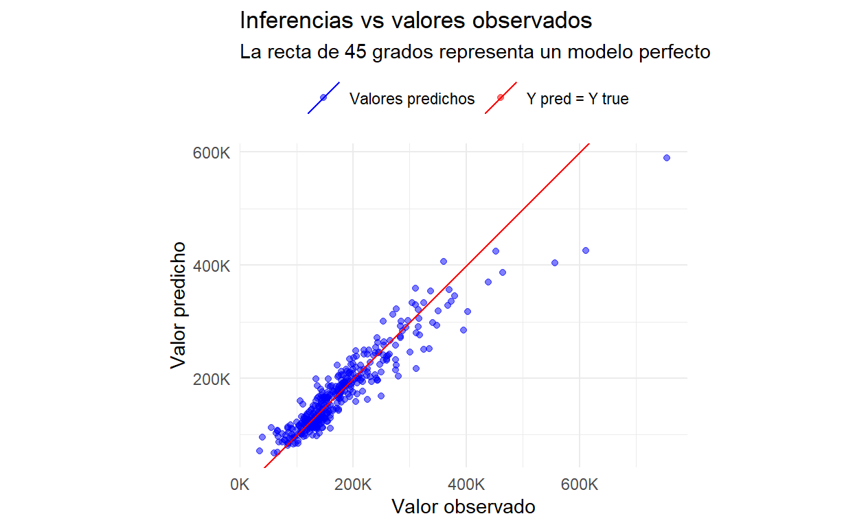

6. Ajuste de hiperparámetros en pipelines 📈

En esta sección se utilizarán 3 técnicas de ajuste de hiperparámetros:

Grid search
Random search
Bayesian search

Se define un preprocesador inicial:

preprocessor = Pipeline([
  ('Preprocesamiento inicial', ColumnTransformer([
    ('numericas', numerical_preprocessor, vars_numericas),
    ('categoricas', categorical_preprocessor, vars_categoricas),
  ], remainder='drop')
  )
])

En este caso, se ajustarán hiperparámetros de 2 modelos:

Light GBM
Random Forest

Se definen ambos modelos:

modelo_lgbm = TransformedTargetRegressor(
  regressor= LGBMRegressor(random_state = 42), 
  func=np.log, 
  inverse_func=np.exp
)

modelo_rf = TransformedTargetRegressor(
  regressor= RandomForestRegressor(random_state=42),
  func=np.log, 
  inverse_func=np.exp
)

Se genera un pipeline que incluye un estimador “dummy”. Este estimador no será ajustado, se modificará por cada uno de los modelos.

class DummyEstimator(BaseEstimator):
    def fit(self): pass
    def score(self): pass

pipe = Pipeline([
    ('preprocesamiento', preprocessor), 
    ('seleccion_vars',    seleccion_vars),
    ('modelo',           DummyEstimator())
])

Los parámetros se configuran como una lista de diccionarios. Dentro del primero componente de la lista de params se incluye la configuración del primer modelo. En este caso, este es un modelo del tipo Random Forest. El segundo diccionario corresponde al segundo modelo, en este caso, un Light GBM.

Show code

p_seleccion_vars = [15,100]
p_max_depth = [4,20]
p_n_estimators = [50,500]
p_min_samples_split = [20,100]
p_num_leaves = [10,100]
p_learning_rate = [0.0001,0.1]

params_grid = [
    {
        'seleccion_vars__k':                     p_seleccion_vars,
        'modelo':                                [modelo_lr],  
    },
    {
        'seleccion_vars__k':                     p_seleccion_vars,
        'modelo':                                [modelo_rf],  
        'modelo__regressor__min_samples_split' : p_min_samples_split,
        'modelo__regressor__max_depth':          p_max_depth,
        'modelo__regressor__n_estimators' :      p_n_estimators,
    },
    {
        'seleccion_vars__k':                     p_seleccion_vars,
        'modelo':                                [modelo_lgbm],
        'modelo__regressor__num_leaves' :        p_num_leaves,
        'modelo__regressor__max_depth' :         p_max_depth,
        'modelo__regressor__learning_rate':      p_learning_rate,
        'modelo__regressor__n_estimators' :      p_n_estimators
    },
]


params_random = [
  {
    'seleccion_vars__k':                         p_seleccion_vars,
    'modelo':                                    [modelo_lr],  
  },  
  {
        'seleccion_vars__k' :                    sp_randInt(p_seleccion_vars[0],p_seleccion_vars[1]),
        'modelo':                                [modelo_rf], 
        'modelo__regressor__max_depth':          sp_randInt(p_max_depth[0],p_max_depth[1]),
        'modelo__regressor__n_estimators':       sp_randInt(p_n_estimators[0],p_n_estimators[1]),
        'modelo__regressor__min_samples_split':  sp_randInt(p_min_samples_split[0],p_min_samples_split[1]),
    },
    {
        'seleccion_vars__k':                     sp_randInt(p_seleccion_vars[0],p_seleccion_vars[1]),
        'modelo':                                [modelo_lgbm],
        'modelo__regressor__num_leaves':         sp_randInt(p_num_leaves[0],p_num_leaves[1]),
        'modelo__regressor__max_depth':          sp_randInt(p_max_depth[0],p_max_depth[1]),
        'modelo__regressor__learning_rate':      st.uniform(p_learning_rate[0],p_learning_rate[1]),
        'modelo__regressor__n_estimators':       sp_randInt(p_n_estimators[0],p_n_estimators[1]),
}]




params_bayes = [
    {
        'seleccion_vars__k':                     p_seleccion_vars,
        'modelo':                                [modelo_lr],  
    },
    {
        'seleccion_vars__k':                     Integer(p_seleccion_vars[0],p_seleccion_vars[1]),
        'modelo':                                [modelo_rf],  
        'modelo__regressor__min_samples_split' : Integer(p_min_samples_split[0],p_min_samples_split[1]),
        'modelo__regressor__max_depth':          Integer(p_max_depth[0],p_max_depth[1]),
        'modelo__regressor__n_estimators' :      Integer(p_n_estimators[0],p_n_estimators[1]),
    },
    {
        'seleccion_vars__k' :                    Integer(p_seleccion_vars[0],p_seleccion_vars[1]),
        'modelo':                                [modelo_lgbm],
        'modelo__regressor__num_leaves':         Integer(p_num_leaves[0],p_num_leaves[1]),
        'modelo__regressor__max_depth' :         Integer(p_max_depth[0],p_max_depth[1]),
        'modelo__regressor__learning_rate':      Real(p_learning_rate[0],p_learning_rate[1]),
        'modelo__regressor__n_estimators' :      Integer(p_n_estimators[0],p_n_estimators[1]),
    },
]

a. Grid search

Dados los parámetros definidos anteriormente, se ajustan N modelos para cubrir todas las combinaciones posibles de parámetros. Esta ténica se denomina grid search.

Pipeline

Se utiliza la técnica de cross-validation, para obtener métricas promedio en cada partición. Notar que en el objeto Pipeline aparece el DummyEstimator().

grid_search = GridSearchCV(pipe, 
    params_grid, 
    n_jobs=1, 
    cv=CV_FOLDS, 
    verbose=0, 
    scoring={"RMSE": "neg_root_mean_squared_error", 
             "MAE" : "neg_mean_absolute_error", 
              "R2": 'r2'},
    refit = "RMSE"
)

grid_search.fit(X_train, y_train)

Mejor modelo

Al seleccionar el mejor modelo en base a la métrica seleccionada, se observa el Pipeline final, en donde quedan definidos los parámetros que maximizan la métrica.

pipe.set_params(**grid_search.best_params_)

Se define una función para obtener las métricas de evaluación de cada uno de los modelos ajustados:

Show code

def eval_metrics(eval_cv):
    eval = (pd.DataFrame(eval_cv.cv_results_)
        .sort_values('mean_test_RMSE', ascending=False)
        .head(20)
        .assign(params = lambda x: x['params'].astype(str))
    )
    return eval

eval_df = eval_metrics(eval_cv=grid_search)

Show code

eval_metrics_table <- function(eval_df){
  eval_df %>%
    mutate(params = str_extract(params, "(?<=regressor=)(.*)(?=\\()")) %>%
    select(params,
           mean_test_RMSE, std_test_RMSE, 
           mean_test_MAE, std_test_MAE,
           mean_test_R2, std_test_R2, 
           starts_with('param_modelo__')) %>% 
    gt() %>% 
    tab_header(title='Modelos según performance') %>% 
    opt_align_table_header('left') 
}

eval_metrics_table(py$eval_df)

params	mean_test_RMSE	std_test_RMSE	mean_test_MAE	std_test_MAE	mean_test_R2	std_test_R2	param_modelo__regressor__max_depth	param_modelo__regressor__min_samples_split	param_modelo__regressor__n_estimators	param_modelo__regressor__learning_rate	param_modelo__regressor__num_leaves
Modelos según performance
LGBMRegressor	-31534.34	6544.146	-17737.07	2064.267	0.8229010	0.08941568	20	NaN	50	0.1	10
LGBMRegressor	-31645.81	6505.232	-17514.05	2276.564	0.8226587	0.08522100	20	NaN	50	0.1	100
LGBMRegressor	-31937.90	6653.572	-18086.26	2116.086	0.8173336	0.09553764	4	NaN	50	0.1	100
LGBMRegressor	-31940.42	7269.146	-17879.61	1958.325	0.8157498	0.10337863	20	NaN	500	0.1	10
LGBMRegressor	-32321.44	6522.782	-18188.14	1967.613	0.8143378	0.09182510	4	NaN	50	0.1	10
LGBMRegressor	-32495.91	8147.759	-18122.75	2211.496	0.8057828	0.12152572	4	NaN	500	0.1	100
LGBMRegressor	-33178.88	8130.031	-18046.53	1953.752	0.7989809	0.12148041	4	NaN	500	0.1	10
LGBMRegressor	-33472.52	5892.323	-20126.86	2534.988	0.8013232	0.09178957	20	NaN	50	0.1	100
LGBMRegressor	-33517.09	6299.600	-20241.14	2770.518	0.7998432	0.09757675	4	NaN	50	0.1	100
RandomForestRegressor	-33618.10	5806.710	-19311.32	2281.548	0.8043264	0.07405322	20	20	500	NaN	NaN
LGBMRegressor	-33685.24	7603.893	-18162.62	2188.372	0.7948441	0.11652537	20	NaN	500	0.1	100
LGBMRegressor	-33709.80	6348.574	-20129.63	2697.037	0.7975307	0.09874874	20	NaN	50	0.1	10
RandomForestRegressor	-33869.83	6036.686	-19323.23	2205.647	0.8024913	0.07083705	20	20	50	NaN	NaN
LGBMRegressor	-33902.11	6307.342	-20158.72	2709.534	0.7954829	0.09924509	4	NaN	50	0.1	10
RandomForestRegressor	-34940.87	5798.645	-20968.64	2606.763	0.7871504	0.08520106	20	20	500	NaN	NaN
RandomForestRegressor	-35019.64	5365.333	-21049.48	2476.029	0.7866916	0.08101604	20	20	50	NaN	NaN
LGBMRegressor	-35167.54	6074.831	-21121.34	2383.424	0.7810622	0.09856842	4	NaN	500	0.1	100
LGBMRegressor	-35398.22	5782.302	-20896.51	1992.189	0.7775885	0.10127984	4	NaN	500	0.1	10
LGBMRegressor	-35408.70	6281.672	-21096.37	2132.609	0.7765633	0.10661069	20	NaN	500	0.1	10
LGBMRegressor	-36079.37	6442.096	-21765.14	2246.711	0.7684244	0.10996980	20	NaN	500	0.1	100

Finalmente, se ajusta el modelo con todos los datos de entrenamiento obteniendo una métrica en la partición de evaluación:

pipe.fit(X_train, y_train)

y_pred = pipe.predict(X_test)
regression_results(y_test, y_pred)

R^2 : 0.88
MAE : 16750.45
RMSE: 29465.78

A partir del pipeline, es posible obtener la importancia de las variables:

feature_imp = pd.DataFrame({
    'variable': pipe[:-1].get_feature_names_out(),
    'feature_imp': pipe['modelo'].regressor_.feature_importances_}
    ).sort_values('feature_imp', ascending=False).head(5)

Show code

py$feature_imp %>% gt() %>% 
  tab_header(title='Importancia de variables (principales 5)')

variable	feature_imp
Importancia de variables (principales 5)
numericas__GrLivArea	61
numericas__OverallCond	32
numericas__YearBuilt	32
numericas__LotArea	28
numericas__BsmtFinSF1	28

b. Random search

Esta técnica permite explorar un conjunto aleatorio de parámetros. Se definen distribuciones para cada uno de los parámetros de cada modelo. El proceso continúa hasta cubrir las N iteraciones aleatorias.

Pipeline

random_search = RandomizedSearchCV(pipe, 
    params_random, 
    n_iter=ITERS, 
    n_jobs=1, 
    cv=CV_FOLDS, 
    verbose=1, 
    scoring={"RMSE": "neg_root_mean_squared_error", 
             "MAE" : "neg_mean_absolute_error", 
              "R2": 'r2'},
    refit = "RMSE"
)

random_search.fit(X_train, y_train)

Mejor modelo

pipe.set_params(**random_search.best_params_)

eval_df = eval_metrics(eval_cv=random_search)

eval_metrics_table(py$eval_df)

params	mean_test_RMSE	std_test_RMSE	mean_test_MAE	std_test_MAE	mean_test_R2	std_test_R2	param_modelo__regressor__learning_rate	param_modelo__regressor__max_depth	param_modelo__regressor__n_estimators	param_modelo__regressor__num_leaves	param_modelo__regressor__min_samples_split
Modelos según performance
LGBMRegressor	-31484.54	6568.184	-17717.71	2352.893	0.8244156	0.08535555	0.02695398	10	163	14	NaN
LGBMRegressor	-31757.01	5931.128	-17744.79	2305.442	0.8236508	0.07457921	0.03033441	7	129	91	NaN
LGBMRegressor	-32008.08	7318.675	-17607.18	2271.754	0.8143502	0.10621544	0.06487983	6	217	13	NaN
LGBMRegressor	-32128.27	5905.586	-19035.97	2179.320	0.8170381	0.08595376	0.01961171	18	231	95	NaN
LGBMRegressor	-32273.59	6686.941	-18088.12	2151.604	0.8136785	0.09714654	0.02309554	11	332	15	NaN
LGBMRegressor	-32302.21	6119.196	-18375.86	2090.281	0.8159546	0.08459057	0.01886969	14	261	91	NaN
LGBMRegressor	-32808.76	6946.754	-18398.78	2229.358	0.8062808	0.10533940	0.02352962	15	429	74	NaN
LGBMRegressor	-32816.06	7717.082	-17831.46	2611.900	0.8048356	0.11261006	0.07989673	8	291	39	NaN
LGBMRegressor	-32852.04	6991.375	-18293.66	2367.615	0.8061065	0.10418349	0.06362707	8	217	64	NaN
LGBMRegressor	-32882.09	6784.410	-18449.25	2013.068	0.8060450	0.10283176	0.08418313	19	112	52	NaN
LGBMRegressor	-33175.45	7337.818	-18486.45	2344.817	0.8011879	0.11177221	0.0556016	7	224	65	NaN
LGBMRegressor	-33310.16	7347.800	-18605.01	2280.512	0.8010677	0.10586333	0.06032226	6	369	22	NaN
LGBMRegressor	-33350.16	7527.247	-18015.71	2250.870	0.7981989	0.11697695	0.07702215	17	439	56	NaN
LGBMRegressor	-33536.59	7199.910	-18658.05	2252.466	0.7969091	0.11251423	0.04917791	7	262	40	NaN
LGBMRegressor	-33645.13	6810.629	-19179.77	2126.785	0.7977392	0.10406316	0.02197966	12	442	37	NaN
LGBMRegressor	-33779.92	6971.724	-18864.17	2025.148	0.7939891	0.11362865	0.04972356	18	426	32	NaN
LGBMRegressor	-33860.05	8009.698	-18463.36	2202.893	0.7916048	0.12343319	0.0775774	6	259	10	NaN
LGBMRegressor	-34295.31	7300.736	-19028.46	1965.320	0.7883067	0.11568809	0.05759936	10	377	54	NaN
LGBMRegressor	-34377.42	7677.032	-19844.05	2523.647	0.7852547	0.12450499	0.03473239	19	494	41	NaN
RandomForestRegressor	-34522.78	5227.291	-20411.73	2029.583	0.7956241	0.06521963	NaN	13	407	NaN	27

Se obtienen las métricas en la partición de evaluación:

pipe.fit(X_train, y_train)

y_pred = pipe.predict(X_test)
regression_results(y_test, y_pred)

R^2 : 0.88
MAE : 16399.47
RMSE: 29280.56

c. Bayesian search

La última técnica a analizar permite, tal como el caso anterior, ajustar N modelos dadas las distribuciones de los parámetros. Sin embargo, en este caso las métricas de modelos anteriores son relevantes para la selección de parámetros en iteraciones siguientes. De esta forma, es una técnica que puede explorar parámetros cercanos a los que maximizan la métrica.

Pipeline

bayes_search = BayesSearchCV(
    pipe,
    search_spaces = params_bayes,
    n_iter=ITERS, 
    cv = CV_FOLDS, 
    n_jobs=1, 
    random_state=42,
    scoring=METRICA
)

bayes_search.fit(X_train, y_train)

Mejor modelo

pipe.set_params(**bayes_search.best_params_)

Métricas en el ajuste de hiperparámetros

Mediante la función plot_objective(), se visualizan los gráficos de dependencia parcial para la función objetivo. Recordar que, en este caso, la métrica a optimizar es el RMSE:

LGBM

Show code

p = plot_objective(
  bayes_search.optimizer_results_[2],
  size=3,
)

plt.show();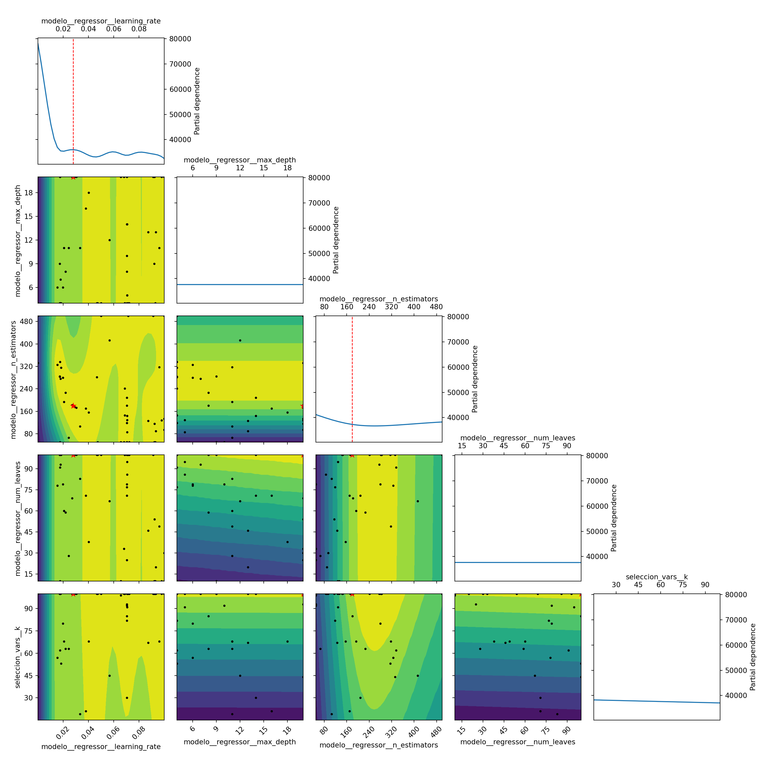

Random Forest

Show code

p = plot_objective(
  bayes_search.optimizer_results_[1],
  size=3,
)

plt.show();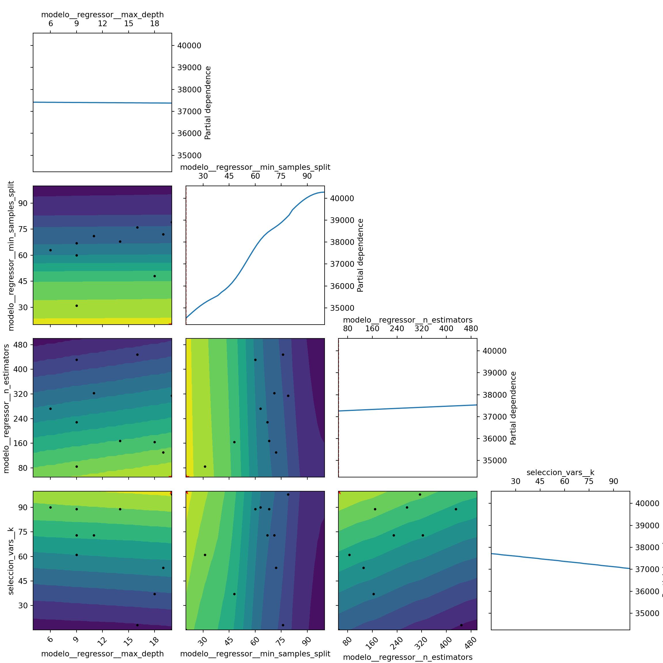

Regresión lineal

Show code

plot_objective(
  bayes_search.optimizer_results_[0], 
  size=8,
)
plt.show();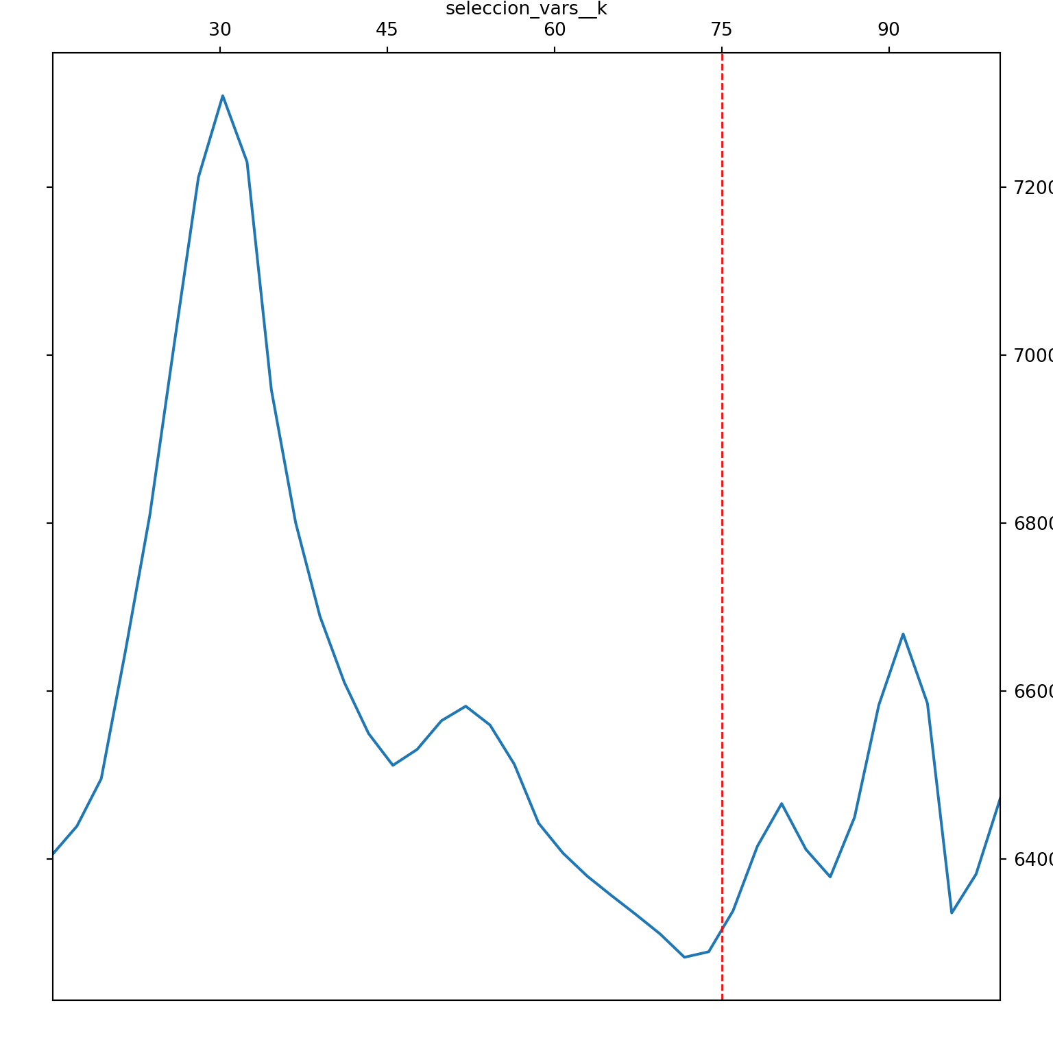

Se observan las métricas de validación cruzada:

eval_df = (pd.DataFrame(bayes_search.cv_results_)
    .sort_values('mean_test_score', ascending=False)
    .assign(params = lambda x: x['param_modelo'].astype(str))
)

Show code

py$eval_df %>% 
  head(10) %>% 
  mutate(params = str_extract(params, "(?<=regressor=)(.*)(?=\\()")) %>%
  select(params,
         mean_test_score,
         std_test_score,
         starts_with('param_modelo__'),) %>%
  gt() %>% 
  tab_header(title='Bayes search: Modelos según performance') %>% 
  opt_align_table_header('left')

params	mean_test_score	std_test_score	param_modelo__regressor__max_depth	param_modelo__regressor__min_samples_split	param_modelo__regressor__n_estimators	param_modelo__regressor__learning_rate	param_modelo__regressor__num_leaves
Bayes search: Modelos según performance
LGBMRegressor	-31239.78	6220.440	20	NaN	179	0.02807448	100
LGBMRegressor	-31309.19	6338.253	20	NaN	182	0.02717604	69
LGBMRegressor	-31330.00	6414.199	20	NaN	176	0.02908675	100
LGBMRegressor	-31412.74	6342.219	9	NaN	284	0.0174014	100
LGBMRegressor	-31426.76	6541.046	7	NaN	276	0.01805463	93
LGBMRegressor	-31446.35	6418.273	20	NaN	173	0.03058374	100
LGBMRegressor	-31499.96	7328.962	20	NaN	133	0.1	10
LGBMRegressor	-31538.94	6844.556	5	NaN	129	0.07055352	95
LGBMRegressor	-31617.92	6744.252	13	NaN	89	0.0933066	20
LGBMRegressor	-31660.01	5478.458	10	NaN	50	0.07053683	79

Show code

metricas = (pd.DataFrame(bayes_search.cv_results_)
  .reset_index().rename({'index':'iteracion'},axis=1)
  .assign(param_modelo = lambda x: x['param_modelo'].astype(str))
)

Visualmente: se observa que en el caso de regresión lineal el desvío es muy grande:

py$metricas %>% 
  mutate(params = str_extract(param_modelo, "(?<=regressor=)(.*)(?=\\()")) %>%
  ggplot(aes(x=iteracion, y=mean_test_score, color=params))+
    geom_line()+
    geom_pointrange(aes(ymin = mean_test_score + std_test_score, 
                        ymax = mean_test_score - std_test_score))+
    labs(color='', x='Iteración', y='Error promedio (CV)')+
    theme(legend.position = 'bottom')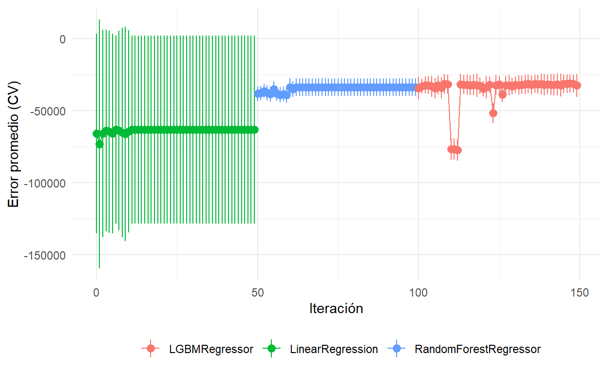

Se obtienen las métricas en la partición de evaluación:

pipe.fit(X_train, y_train)

y_pred = pipe.predict(X_test)
regression_results(y_test, y_pred)

R^2 : 0.88
MAE : 16281.4
RMSE: 28859.42

Comentarios finales

En este post se hizo uso de diversas técnicas de optimización de hiperparámetros mediante la implementación de pipelines de sklearn. No se buscaba mejorar la métrica, solo ilustrar las posibilidades de uso. Cualquier comentario es bienvenido!

Contacto ✉

Karina Bartolome, Linkedin, Twitter, Github, Blogpost

Pedregosa, F., G. Varoquaux, A. Gramfort, V. Michel, B. Thirion, O. Grisel, M. Blondel, et al. 2011. “Scikit-Learn: Machine Learning in Python.” Journal of Machine Learning Research 12: 2825–30.

Pedregosa et al. (2011)↩︎

Comment on this article

Pipelines en Scikit-Learn

Introducción

Conda environment 🐍

Librerías 📚

1. Datos 📊

2. Partición en train y test ✂️

3. Pipeline de preprocesamiento ⚙️

4. Modelado simple 📓

5. Pipeline de preprocesamiento + modelado 💡

6. Ajuste de hiperparámetros en pipelines 📈

a. Grid search

Pipeline

Mejor modelo

b. Random search

Pipeline

Mejor modelo

c. Bayesian search

Pipeline

Mejor modelo

Métricas en el ajuste de hiperparámetros

LGBM

Random Forest

Regresión lineal

Comentarios finales

Contacto ✉

References

Citation