Maine
This article shows the application of Workflowsets to time series analysis, through the package sknifedatar. It is an extension of the Modeltime ecosystem. The presented use case corresponds to USgas package data: US monthly natural gas consumption by residential consumers by state and aggregate level between 1989 and 2020.
Workflowsets1 📦 is a recent tidymodels2 📦 package that allows to create and easily fit combinations of preprocessors (e.g., formula, recipe, etc) and model specifications.
Using this tidy approach we’ve developed an adaptation that allows us to extend the use of workflowsets to the analysis of time series. The connection is made through the sknifedatar3 📦 package (that serves primarily as an extension to the modeltime framework), which allows linking the modeltime4 ecosystem with workflowsets.
At a general level, this is the modeling scheme:
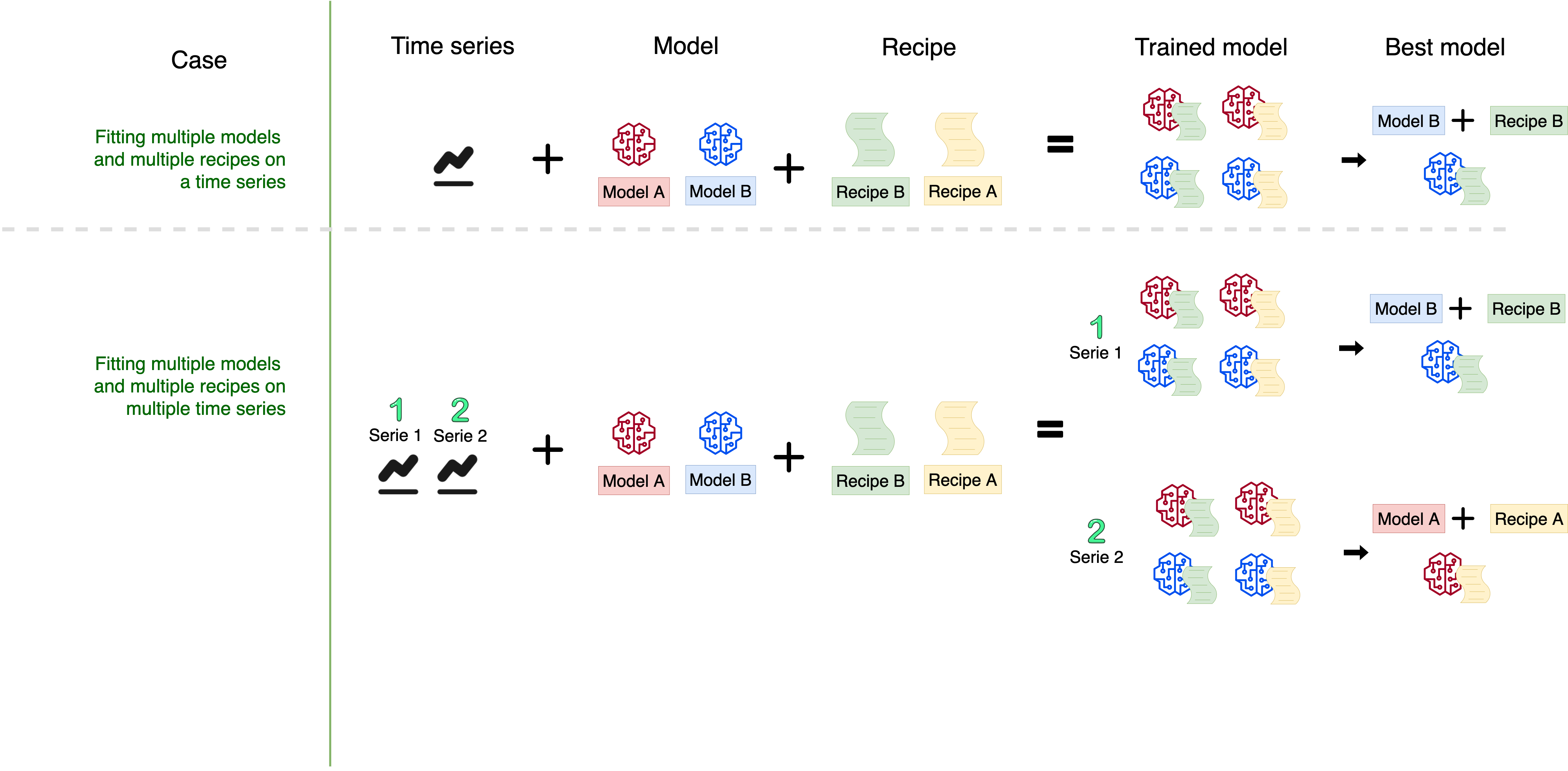
This article includes a new sknifedatar functionality. The fitting of a Workflowset on multiple time series 🤩 (individual series, not panel), with an approach similar to that of our previous publication, Multiple Models Over Multiple Time Series: A Tidy Approach.
The necessary libraries are imported.
For data manipulation we used the tidyverse5 📦 ecosystem.
For this example, time series data from the US monthly natural gas consumption by residential consumers by state and aggregate level between 1989 and 2020 is used. This data is available in the USgas6 package 📦.
data_states <-  USgas::us_residential %>% rename(value=y) %>%
  filter(date <='2020-09-01')
🔹 The dataset includes data for the following states:
Alabama, Alaska, Arizona, Arkansas, California, Colorado, Connecticut, Delaware, District of Columbia, Florida, Georgia, Hawaii, Idaho, Illinois, Indiana, Iowa, Kansas, Kentucky, Louisiana, Maine, Maryland, Massachusetts, Michigan, Minnesota, Mississippi, Missouri, Montana, Nebraska, Nevada, New Hampshire, New Jersey, New Mexico, New York, North Carolina, North Dakota, Ohio, Oklahoma, Oregon, Pennsylvania, Rhode Island, South Carolina, South Dakota, Tennessee, Texas, U.S., Utah, Vermont, Virginia, Washington, West Virginia, Wisconsin and Wyoming
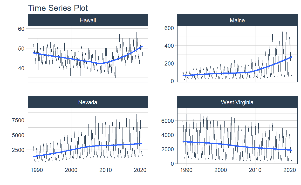
We’ve decided to select Nevada, Maine, Hawaii and West Virginia, since gas consumption has not been as homogeneous among them, this allows us to better understand the use case of time series adjustment of models.
👉 In this article we will focus on one of these series. In the next section we will focus on the rest of them.
data_states <- data_states %>%
  filter(state %in%  c('Nevada','Hawaii','West Virginia','Maine'))

data_states %>%
  group_by(state) %>%
  plot_time_series(.date_var = date,
                   .value=value,
                   .facet_ncol = 2,
                   .line_size = 0.2,
                   .interactive = FALSE
  )
In this first case, a set of models and preprocessors are fitted to an individual series.
The first 5 rows are displayed. Notice that it’s a monthly series.
| US monthly consumption of natural gas by residential consumers by state and aggregate level between 1989 and 2020 | |
| Units: Million Cubic Feet | |
| date | value |
|---|---|
| 1989-01-01 | 51 |
| 1989-02-01 | 52 |
| 1989-03-01 | 50 |
| 1989-04-01 | 50 |
| 1989-05-01 | 47 |
The time series partition ➗ on train and test is shown below:
initial_time_split(data = data, prop = 0.8) %>%
  tk_time_series_cv_plan() %>%
  plot_time_series_cv_plan(date, value, .interactive = FALSE,
                           .title = "Hawaii - Partition Train / Test") +
  theme(strip.text = element_blank())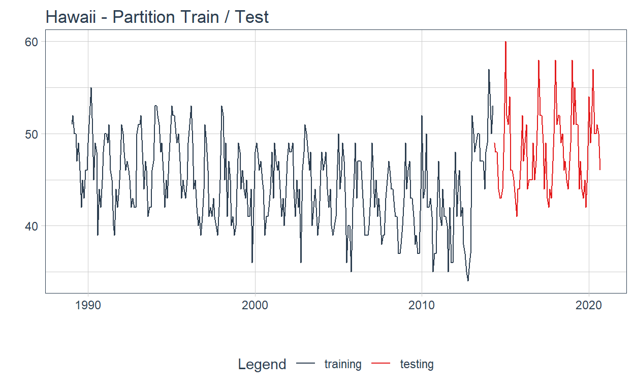
📌 The transformation recipes are defined following the 🌟 Tidymodels framework 🌟.
🔹recipe_base: base recipe, representing the base preprocessing specification, where the formula is \(value=f(date)\).
🔹recipe_date_features: base_recipe + some additional features generated from the date column: ‘month’,‘year’.
🔹recipe_date_extrafeatures: recipe_date_features + more additional features from the date column: ‘quarter’,‘semester’.
🔹recipe_date_extrafeatures_lag: recipe_date_extrafeatures + 6 lagged columns including lagged values. The NA values for the first observations, where no lagged values can be computed, are imputed with a time series imputation step.
🔹recipe_base_fourier: fourier transformation applied to the date feature.
# Recipe without steps, just imputation of missing values
recipe_base <- recipe(value~date, data=data) %>%
    step_ts_impute(all_numeric(), period=365)

# Some date variables
recipe_date_features <- recipe_base %>%
  step_date(date, features = c('month','year'))

# More date variables
recipe_date_extrafeatures <- recipe_date_features %>%
  step_date(date, features = c('quarter','semester'))

# Lagged values: 1 to 6 months lag
recipe_date_extrafeatures_lag <- recipe_date_extrafeatures %>%
  step_lag(value, lag = 1:6) %>%
  step_ts_impute(all_numeric(), period=365)

# Fourier transformation
recipe_date_extrafeatures_fourier <-recipe_date_extrafeatures  %>%
step_fourier(date, period = 365/12, K = 1)📌 Below are the models that will be fitted.
🔹auto_arima_boost: a automatic ARIMA boosted model specification.
🔹prophet_boost: a prophet model specification.
🔹prophet_boost_log: a prophet model specification with logarithmic growth.
🔹mars: a Multivariate Adaptive Regression Splines model specification.
🔹nnetar: a Neural network time series model specification.
# prophet_xgboost
prophet_boost <- prophet_boost(mode = 'regression') %>%
  set_engine("prophet_xgboost")

# prophet_xgboost logistic
prophet_boost_log <- prophet_boost(
    mode = 'regression',
    changepoint_range = 0.8,
    logistic_floor = min(data$value),
    logistic_cap = max(data$value),
    growth = 'logistic'
  ) %>%
  set_engine("prophet_xgboost")

# mars
mars <- mars( mode = 'regression') %>%
  set_engine('earth')

# nnetar
nnetar <- nnetar_reg() %>%
  set_engine("nnetar")

#auto_arima_xgboost
auto_arima_boost <- arima_boost() %>%
set_engine('auto_arima_xgboost')⚙️ Through Workflowsets we can automatically fit all possible combinations of models and recipes. Here we are adapting workflowsets to modeltime, for the original workflowsets application see: workflowsets 0.0.1
wfsets <- workflow_set(
  preproc = list(
    base                  = recipe_base,
    features              = recipe_date_features,
    extrafeatures         = recipe_date_extrafeatures,
    extrafeatures_lag     = recipe_date_extrafeatures_lag,
    extrafeatures_fourier = recipe_date_extrafeatures_fourier
  ),
  models  = list(
    M_arima_boost       = auto_arima_boost,
    M_prophet_boost_log = prophet_boost_log,
    M_prophet_boost     = prophet_boost,
    M_mars              = mars,
    M_nnetar            = nnetar
  ),
  cross   = TRUE
)
wfsets
# A workflow set/tibble: 25 × 4
wflow_id info option result
<chr> <list> <list> <list>
1 base_M_arima_boost <tibble [1 × 4]> <opts[0]> <list [0]>
2 base_M_prophet_boost_log <tibble [1 × 4]> <opts[0]> <list [0]>
3 base_M_prophet_boost <tibble [1 × 4]> <opts[0]> <list [0]>
4 base_M_mars <tibble [1 × 4]> <opts[0]> <list [0]>
5 base_M_nnetar <tibble [1 × 4]> <opts[0]> <list [0]>
6 features_M_arima_boost <tibble [1 × 4]> <opts[0]> <list [0]>
7 features_M_prophet_boost_log <tibble [1 × 4]> <opts[0]> <list [0]>
8 features_M_prophet_boost <tibble [1 × 4]> <opts[0]> <list [0]>
9 features_M_mars <tibble [1 × 4]> <opts[0]> <list [0]>
10 features_M_nnetar <tibble [1 × 4]> <opts[0]> <list [0]>
# ℹ 15 more rows📝 Since the models nnetar and mars have a strange behavior when including lags, we have decided not to include them in the models to fit. To remove models from the wfsets object it is possible to use the anti_join() function from dplyr 📦
Through modeltime_wfs_fit, a function included in sknifedatar 📦, a workflowsets object including time series workflows can be fitted on an individual series. This function only requires the workflowsets object, the time series split proportion and the time series.
set.seed(1234)
split_prop <- 0.8
wffits <- modeltime_wfs_fit(.wfsets = wfsets,
                            .split_prop = split_prop,
                            .serie=data)
wffits %>% head(2)
Observing the object wfftis, it can be seen that all metrics corresponing to each combination of recipes with models are displayed. Also, the model fitted is stored.
# A tibble: 2 × 10
  .model_id     .model_desc .type   mae  mape  mase smape  rmse    rsq
  <chr>         <chr>       <chr> <dbl> <dbl> <dbl> <dbl> <dbl>  <dbl>
1 base_M_arima… ARIMA(0,1,… Test   4.74  10.1  1.46  9.46  5.40 0.599
2 base_M_mars   EARTH       Test  13.3   28.3  4.09 24.2  14.7  0.0223
# ℹ 1 more variable: .fit_model <list>
🔹 This object is displayed below in a well formatted table. Notice that the .fit_model column is excluded for better visualization.
wffits %>%
  select(-.fit_model, -.model_desc, -.type) %>%
  separate(.model_id, c('recipe', 'model'), sep='_M_', remove=FALSE) %>%
  arrange(desc(rsq)) %>%
  gt() %>%
  tab_header(title='Models sets evaluation') %>%
  tab_footnote(
    footnote = "Only possible combinations of models with recipes are shown.",
    locations = cells_column_labels(
      columns = c(.model_id))
)| Models sets evaluation | ||||||||
| .model_id1 | recipe | model | mae | mape | mase | smape | rmse | rsq |
|---|---|---|---|---|---|---|---|---|
| base_M_prophet_boost | base | prophet_boost | 2.715799 | 5.498342 | 0.8356304 | 5.686372 | 3.284976 | 6.577389e-01 |
| base_M_prophet_boost_log | base | prophet_boost_log | 5.974799 | 12.193184 | 1.8383997 | 13.111905 | 6.490424 | 6.445390e-01 |
| extrafeatures_M_prophet_boost_log | extrafeatures | prophet_boost_log | 2.274725 | 4.814021 | 0.6999154 | 4.710788 | 2.809709 | 6.187427e-01 |
| features_M_prophet_boost | features | prophet_boost | 3.639383 | 7.856472 | 1.1198103 | 7.454231 | 4.268795 | 6.046994e-01 |
| base_M_arima_boost | base | arima_boost | 4.736744 | 10.086012 | 1.4574596 | 9.457385 | 5.402352 | 5.991789e-01 |
| extrafeatures_lag_M_prophet_boost_log | extrafeatures_lag | prophet_boost_log | 2.201133 | 4.560134 | 0.6772717 | 4.556901 | 2.699579 | 5.970839e-01 |
| extrafeatures_M_prophet_boost | extrafeatures | prophet_boost | 3.439385 | 7.418118 | 1.0582722 | 7.047736 | 4.105563 | 5.962231e-01 |
| extrafeatures_lag_M_prophet_boost | extrafeatures_lag | prophet_boost | 2.774248 | 5.907029 | 0.8536149 | 5.672052 | 3.472725 | 5.923840e-01 |
| features_M_prophet_boost_log | features | prophet_boost_log | 2.493793 | 5.312523 | 0.7673210 | 5.165195 | 3.066893 | 5.864230e-01 |
| extrafeatures_M_arima_boost | extrafeatures | arima_boost | 4.425513 | 9.427621 | 1.3616962 | 8.853871 | 5.159703 | 5.857852e-01 |
| features_M_arima_boost | features | arima_boost | 4.982869 | 10.638650 | 1.5331906 | 9.929374 | 5.733011 | 5.373927e-01 |
| extrafeatures_fourier_M_prophet_boost_log | extrafeatures_fourier | prophet_boost_log | 2.598130 | 5.248098 | 0.7994246 | 5.370895 | 3.303457 | 5.229104e-01 |
| extrafeatures_fourier_M_prophet_boost | extrafeatures_fourier | prophet_boost | 2.394988 | 4.998421 | 0.7369193 | 4.901557 | 3.087135 | 5.151333e-01 |
| extrafeatures_lag_M_arima_boost | extrafeatures_lag | arima_boost | 4.945582 | 10.595702 | 1.5217177 | 9.880220 | 5.728650 | 5.087098e-01 |
| extrafeatures_fourier_M_arima_boost | extrafeatures_fourier | arima_boost | 5.680544 | 12.078615 | 1.7478596 | 11.174632 | 6.556410 | 4.372646e-01 |
| extrafeatures_fourier_M_nnetar | extrafeatures_fourier | nnetar | 4.867873 | 9.990006 | 1.4978072 | 10.636061 | 5.620020 | 4.173088e-01 |
| extrafeatures_M_nnetar | extrafeatures | nnetar | 4.656186 | 9.570021 | 1.4326725 | 10.198180 | 5.548765 | 3.980986e-01 |
| features_M_nnetar | features | nnetar | 4.327944 | 8.997786 | 1.3316750 | 9.443067 | 5.077462 | 3.455357e-01 |
| features_M_mars | features | mars | 22.177297 | 46.187083 | 6.8237838 | 36.122812 | 24.682611 | 1.809680e-01 |
| extrafeatures_fourier_M_mars | extrafeatures_fourier | mars | 22.171107 | 46.176874 | 6.8218791 | 36.116256 | 24.675566 | 1.800414e-01 |
| extrafeatures_M_mars | extrafeatures | mars | 22.228102 | 46.294152 | 6.8394161 | 36.188636 | 24.738947 | 1.798935e-01 |
| base_M_mars | base | mars | 13.307100 | 28.329840 | 4.0944923 | 24.150031 | 14.697895 | 2.230231e-02 |
| base_M_nnetar | base | nnetar | 3.683298 | 7.500538 | 1.1333225 | 7.594745 | 4.617912 | 7.634042e-05 |
| 1 Only possible combinations of models with recipes are shown. | ||||||||
🔹 For each workflow a forecast is made in the test partition. This can be done through the modeltime_wfs_forecast function, also from sknifedatar 📦. Notice that this is an adaptation from the modeltime_forecast function. In order to predict on test data, it is only required to specify the wffits object, the series and the split proportion.
modeltime_wfs_forecast(.wfs_results = wffits,
                       .serie = data,
                       .split_prop=split_prop) %>%
  plot_modeltime_forecast(.interactive=FALSE)+
  theme(legend.direction = 'vertical')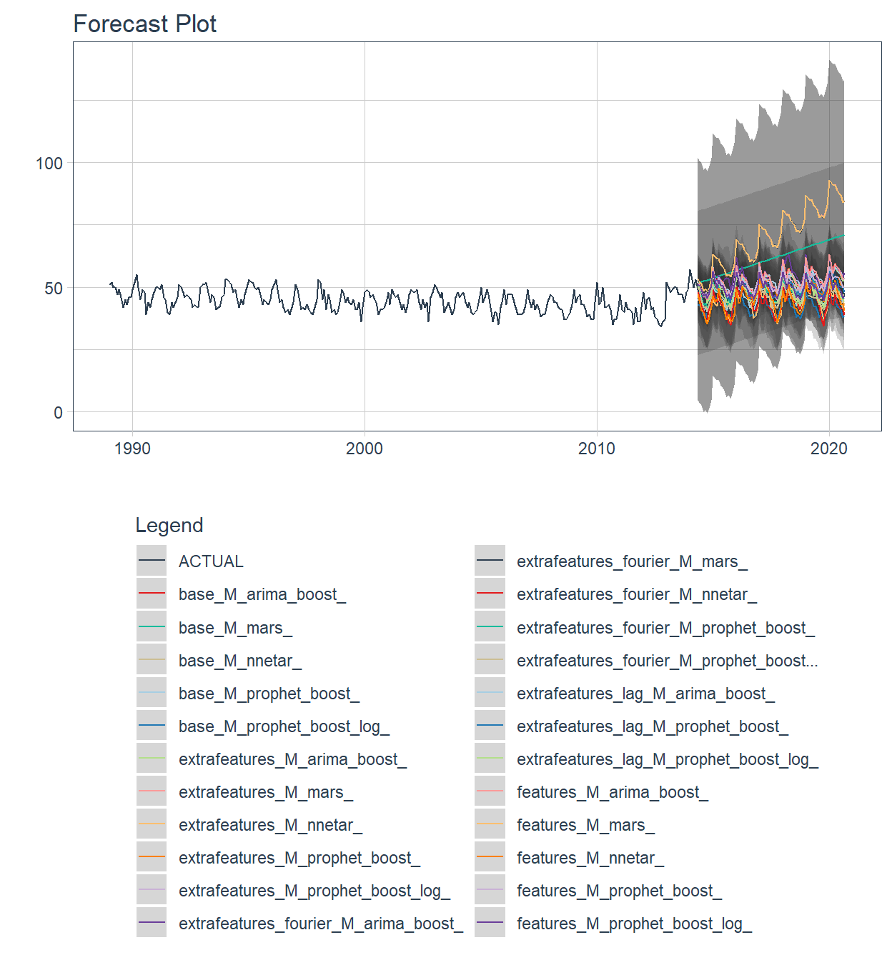
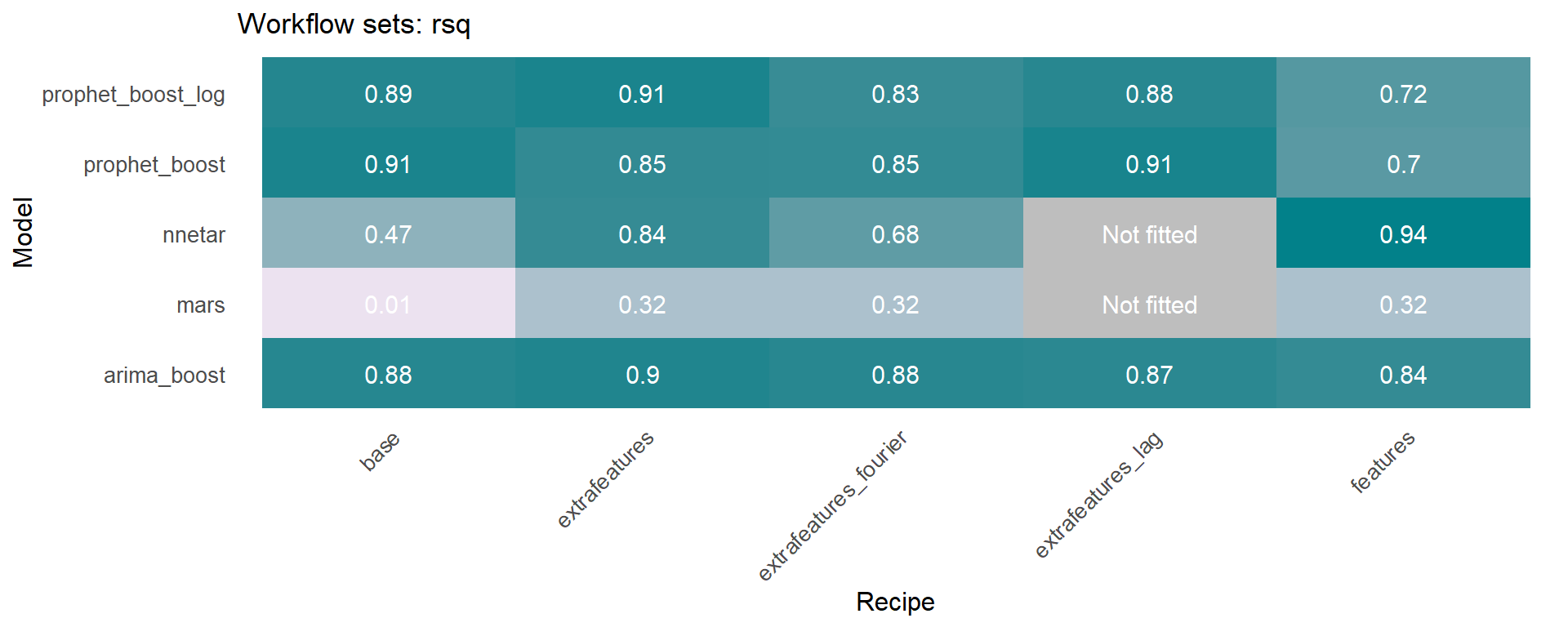
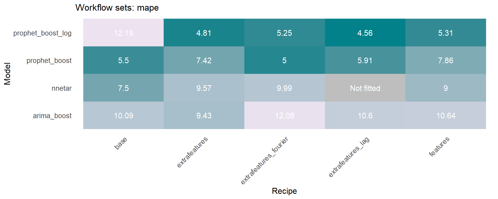
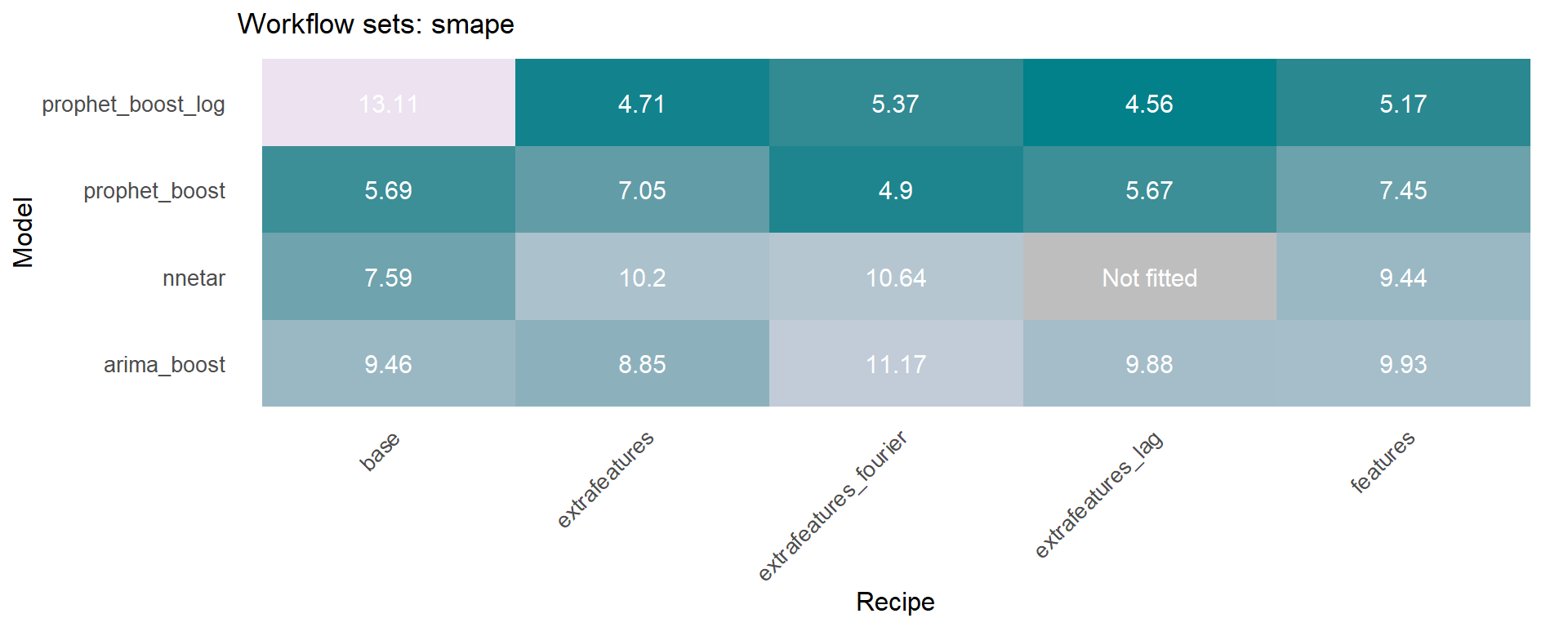
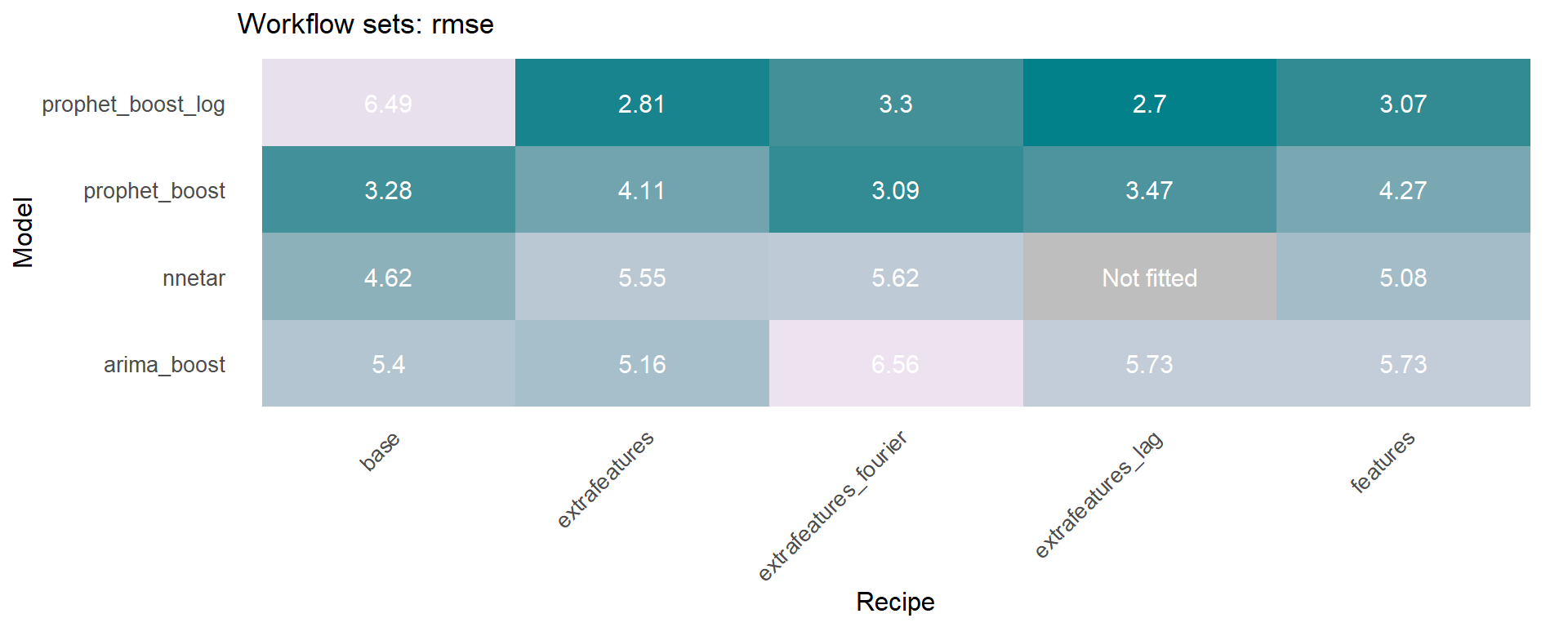
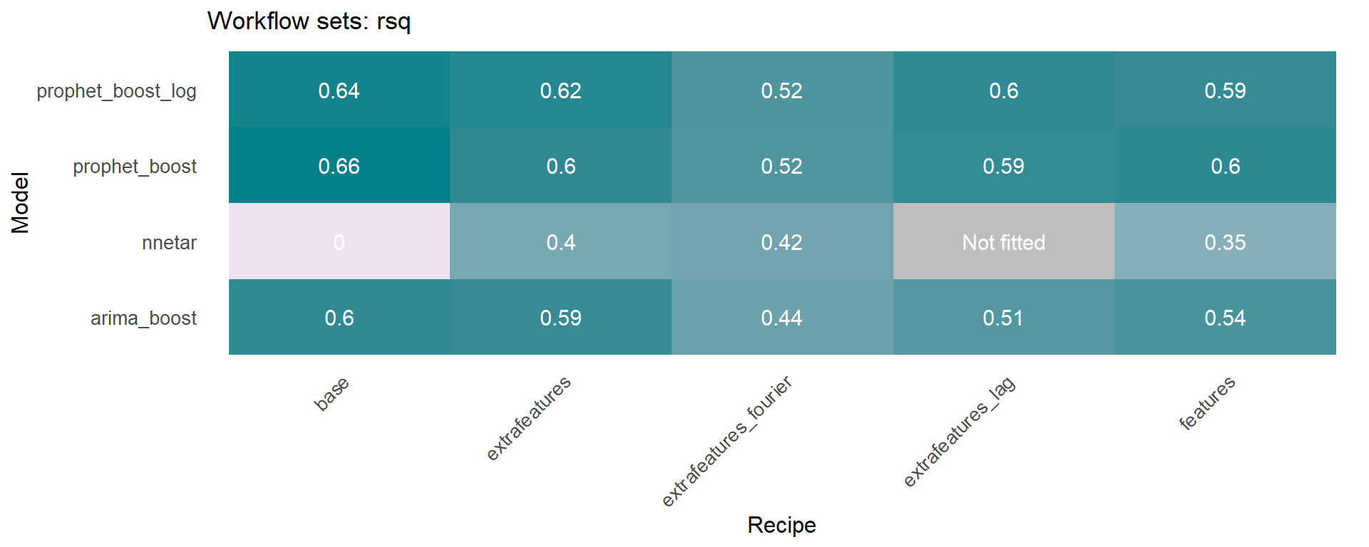
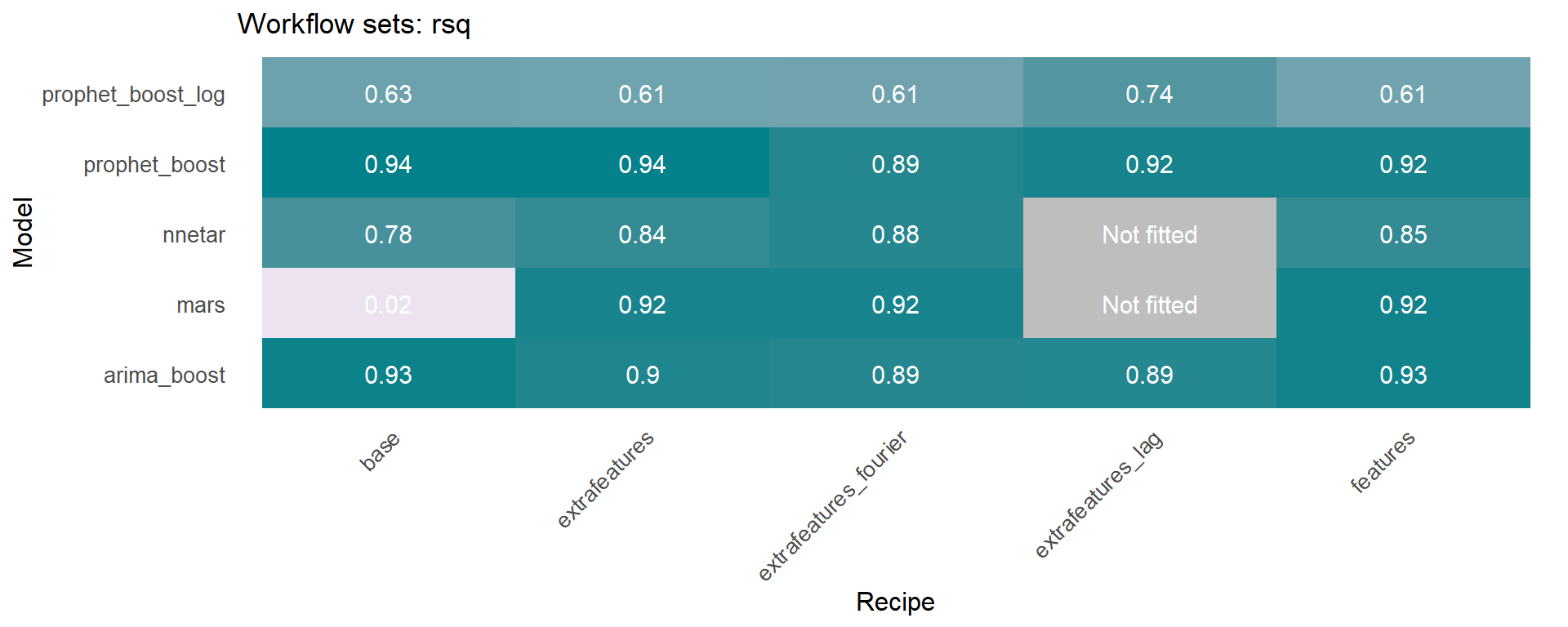
The workflowsets package allows to fit all possible combinations of models and preprocessors. We have included an additional function on the sknifedatar 📦 package. The modeltime_wfs_heatmap allows to easily generate a heatmap for each recipe and model on a wffits object 🙌 generated with the modeltime_wfs_fit function.
The modeltime_accuracy function from modeltime generates 6 time series metrics (‘mae’,‘mape’,‘mase’,‘smape’,‘rmse’,‘rsq’). The modeltime_wfs_heatmap takes as input the selected metric and the adjusted workflows and generates a heatmap.
🚨 We have decided to exclude the MARS model from these heatmaps since it was shown before that the performance was not so good and the color scale of the heatmap works better without this model.
The modeltime_wfs_heatmap was applied to each metric, generating a dataframe that includes a row for each metric and a column that includes the heatmap plot.
heatmap_metrics <-
  data.frame(metric = c('mae', 'mape', 'mase', 'smape', 'rmse', 'rsq')) %>%
  mutate(plot = map(metric,
                    ~ modeltime_wfs_heatmap(.wfs_results = wffits,
                                             metric = .x,
                                             low_color = '#ece2f0',
                                             high_color = '#02818a')
  ))
👉 In order to visualize the heatmaps on tabs, the automagic_tabs function from sknifedatar 📦 is used. For a better understanding of this function, visit: Automagic Tabs in Distill/Rmarkdown files and time series analysis
xaringanExtra::use_panelset()The following chunk is actually executed inline:
#'r automagic_tabs(input_data=temp, panel_name="metric", .output="plot",
#                  echo=FALSE, .layout="l-page", fig.heigth=2, fig.width=10)'

🔹 The modeltime_wfs_rank function from sknifedatar generates a ranking of models generated with modeltime_wfs_fit.
ranking <- modeltime_wfs_rank(wffits,
                              rank_metric = "rsq",
minimize = FALSE)ranking %>% select(.model_id, rank, .model_desc) %>% gt() %>%
tab_header(title='Model ranking') %>%
opt_align_table_header('left')| Model ranking | ||
| .model_id | rank | .model_desc |
|---|---|---|
| base_M_prophet_boost | 1 | PROPHET |
| base_M_prophet_boost_log | 2 | PROPHET |
| extrafeatures_M_prophet_boost_log | 3 | PROPHET W/ XGBOOST ERRORS |
| features_M_prophet_boost | 4 | PROPHET W/ XGBOOST ERRORS |
| base_M_arima_boost | 5 | ARIMA(0,1,3)(0,1,1)[12] |
| extrafeatures_lag_M_prophet_boost_log | 6 | PROPHET W/ XGBOOST ERRORS |
| extrafeatures_M_prophet_boost | 7 | PROPHET W/ XGBOOST ERRORS |
| extrafeatures_lag_M_prophet_boost | 8 | PROPHET W/ XGBOOST ERRORS |
| features_M_prophet_boost_log | 9 | PROPHET W/ XGBOOST ERRORS |
| extrafeatures_M_arima_boost | 10 | ARIMA(0,1,3)(0,1,1)[12] W/ XGBOOST ERRORS |
| features_M_arima_boost | 11 | ARIMA(0,1,3)(0,1,1)[12] W/ XGBOOST ERRORS |
| extrafeatures_fourier_M_prophet_boost_log | 12 | PROPHET W/ XGBOOST ERRORS |
| extrafeatures_fourier_M_prophet_boost | 13 | PROPHET W/ XGBOOST ERRORS |
| extrafeatures_lag_M_arima_boost | 14 | ARIMA(0,1,3)(0,1,1)[12] W/ XGBOOST ERRORS |
| extrafeatures_fourier_M_arima_boost | 15 | ARIMA(0,1,3)(0,1,1)[12] W/ XGBOOST ERRORS |
| extrafeatures_fourier_M_nnetar | 16 | NNAR(1,1,10)[12] |
| extrafeatures_M_nnetar | 17 | NNAR(1,1,10)[12] |
| features_M_nnetar | 18 | NNAR(1,1,10)[12] |
| base_M_nnetar | 19 | NNAR(1,1,10)[12] |
➡️ The best models are selected based on a metric. In order to do this, the modeltime_wfs_bestmodel function is used, which gets the best combination of model and recipe based on a a wffits object generated from the modeltime_wfs_fit function.
This function allows to select workflows on three ways:
.model = “top n”, “Top n” or “tOp n”: where n is the number of best models to select.
.model = n, where n is the number of best models to select.
.model = name of the workflow or workflows to select.
wffits_best <- modeltime_wfs_bestmodel(.wfs_results = ranking,
                                      .model = "top 4",
                                      .metric = "mae",
.minimize = TRUE)wffits_best %>%
select(.model_id, rank, .model_desc) %>% head(5) %>%
gt() %>% tab_header(title='Top 4 models') %>%
opt_align_table_header('left')| Top 4 models | ||
| .model_id | rank | .model_desc |
|---|---|---|
| extrafeatures_lag_M_prophet_boost_log | 1 | PROPHET W/ XGBOOST ERRORS |
| extrafeatures_M_prophet_boost_log | 2 | PROPHET W/ XGBOOST ERRORS |
| extrafeatures_fourier_M_prophet_boost | 3 | PROPHET W/ XGBOOST ERRORS |
| features_M_prophet_boost_log | 4 | PROPHET W/ XGBOOST ERRORS |
👉After selecting the top 4 models, the modeltime_wfs_forecast is used again, but in this case for the best models.
modeltime_wfs_forecast(.wfs_results = wffits_best,
                       .serie = data,
                       .split_prop=split_prop) %>%
  plot_modeltime_forecast(.interactive=FALSE)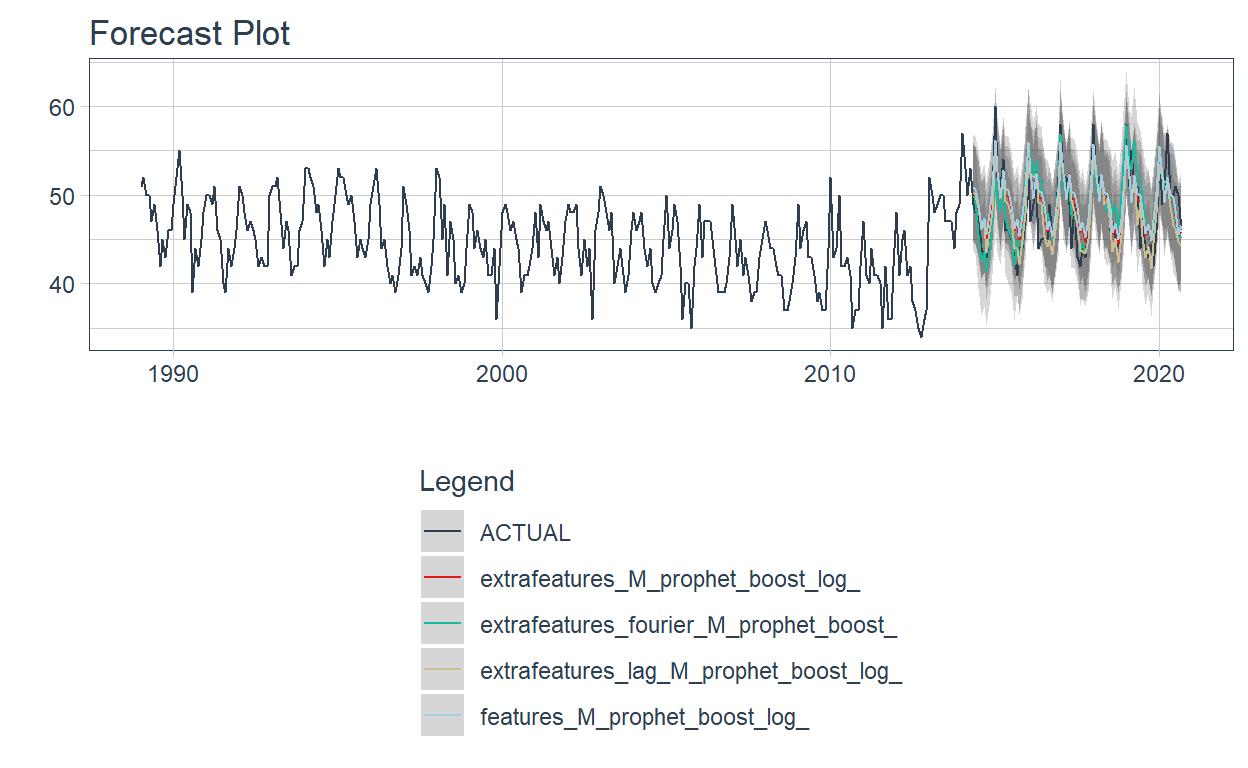
Now the models are re-fitted for the whole dataset (training + testing partitions), through the modeltime_wfs_refit function from sknifedatar.
🔹 This function applies the modeltime_refit() function from modeltime to the wffits object generated from the modeltime_wfs_fit function.
wfrefits <- modeltime_wfs_refit(.wfs_results = wffits_best, .serie = data)
wfrefits
# Modeltime Table
# A tibble: 4 × 3
.model_id .model .model_desc
<chr> <list> <chr>
1 extrafeatures_fourier_M_prophet_boost <workflow> PROPHET W/ XGBOOST…
2 extrafeatures_lag_M_prophet_boost_log <workflow> PROPHET W/ XGBOOST…
3 extrafeatures_M_prophet_boost_log <workflow> PROPHET W/ XGBOOST…
4 features_M_prophet_boost_log <workflow> PROPHET W/ XGBOOST…Now the modeltime_wfs_forecast is used again, but for future forecasting. In order to do this, the .h parameter is included.
wfrefits_forecast <- modeltime_wfs_forecast(.wfs_results = wfrefits,
                                            .serie = data,
                                            .h = '1 year',
                                            .split_prop = split_prop)

wfrefits_forecast %>%
  plot_modeltime_forecast(.interactive=FALSE) +
  theme(legend.direction = 'vertical')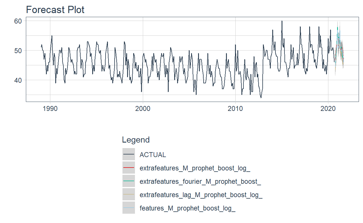
🔹Considering the 4 series selected at the beginning. The first necessary step is to nest the series into a nested dataframe, where the first column is the state, and the second column is the nested_column (date and value).
The modeltime_wfs_multifit function from sknifedatar 📦 allows a 🌟 workflowset object to be fitted over multiple time series 🌟. In this function, the workflow_set object is the same as the one used before, since it contains the diferent model + recipes combinations.
set.seed(1234)
wfs_multifit <- modeltime_wfs_multifit(serie = nested_data,
                                       .prop = 0.8,
                                       .wfs  = wfsets)
👉 The fitted object is a list containing the fitted models (table_time) and the corresponding metrics for each model (models_accuracy).
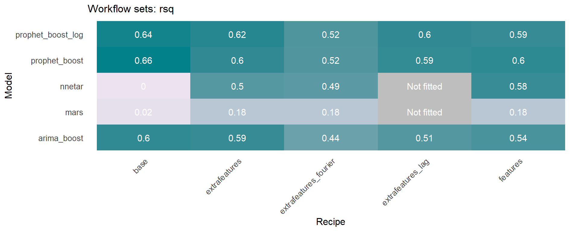
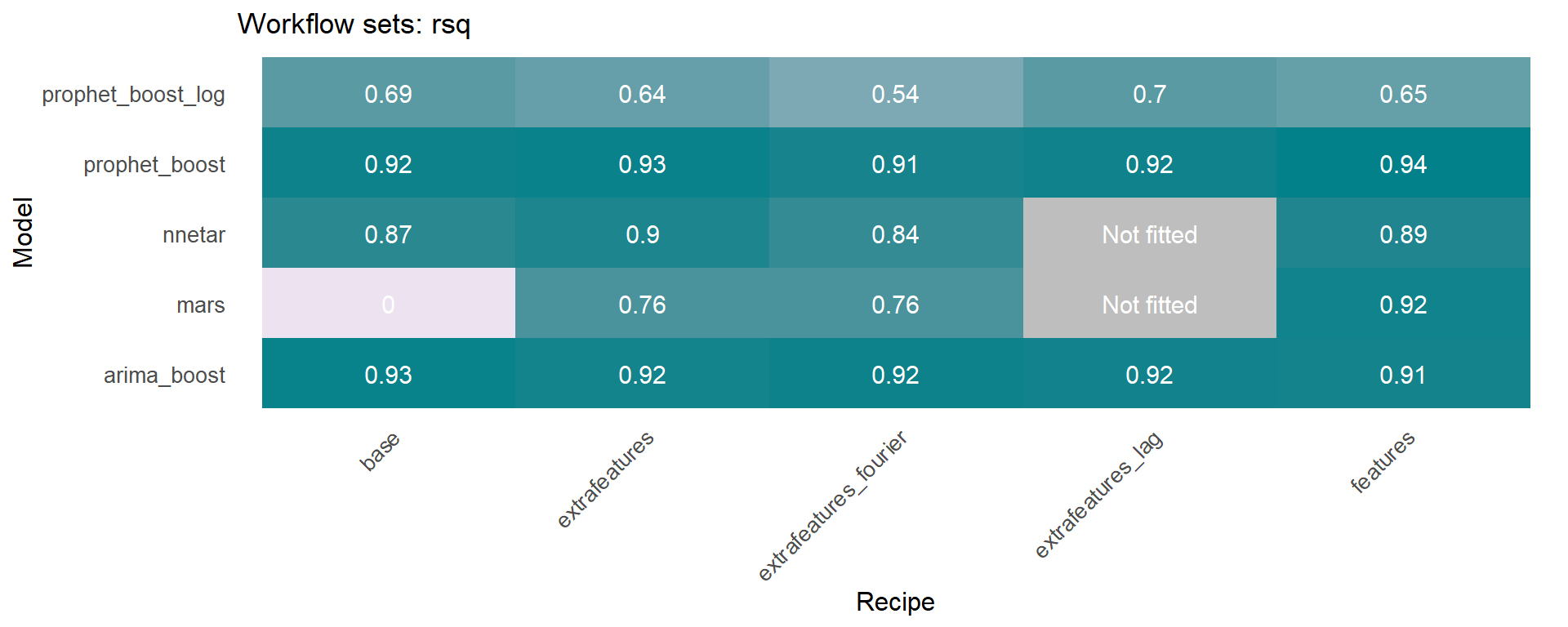
🔹 Using the models_accuracy table included in the wfs_multifit object, a heatmap can be generated for a specific metric for each series 🔍 . This is done using the modeltime_wfs_heatmap function presented above.
Another function included in sknifedatar is modeltime_wfs_multiforecast, which generates 🧙 forecast of a workflow_set fitted object over multiple time series.
wfs_multiforecast <- modeltime_wfs_multiforecast(
  wfs_multifit$table_time, .prop=0.8)
🔹The plot_modeltime_forecast function from modeltime is used to visualize each forecast, where the nested_forecast is unnnested before using the function. As it can be seen, many models did not perform well.
wfs_multiforecast %>%
      select(state, nested_forecast) %>%
      unnest(nested_forecast) %>%
      filter(.model_desc!='base_M_mars') %>%
      group_by(state) %>%
      plot_modeltime_forecast(
        .legend_max_width = 12,
        .facet_ncol = 2,
        .line_size = 0.5,
        .interactive = FALSE,
        .facet_scales = 'free_y',
        .title='Proyecciones') +
  theme(legend.position='bottom')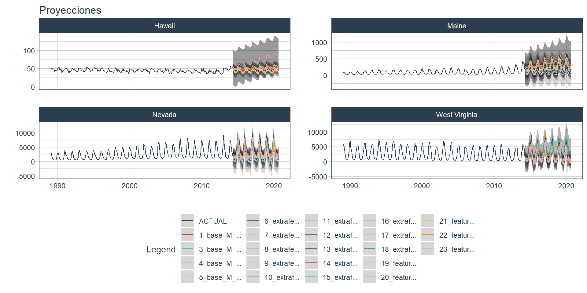
The modeltime_wfs_multibest 🏅 from sknifedatar obtains the best workflow/model for each time series based on a performance metric (one of ‘mae’, ‘mape’,‘mase’, ‘smape’,‘rmse’,‘rsq’).
wfs_bests<- modeltime_wfs_multibestmodel(
      .table = wfs_multiforecast,
      .metric = "rsq",
      .minimize = FALSE
)Now that we’ve selected the best model for each series, the modeltime_wfs_multirefit function is used in order to retrain a set of workflows on all the data (train and test) 👌
set.seed(1234)
wfs_refit <- modeltime_wfs_multirefit(wfs_bests)Finally, a new forecast is generated for the refitted object 🧙, resulting in 4 forecasts, one for each series. In this case, the modeltime_wfs_multiforecast is used with .h paramenter = ‘12 month’, giving a future forecast.
wfs_forecast <- modeltime_wfs_multiforecast(wfs_refit, .h = "12 month")

wfs_forecast %>%
      select(state, nested_forecast) %>%
      unnest(nested_forecast) %>%
      group_by(state) %>%
      plot_modeltime_forecast(
        .legend_max_width = 30,
        .facet_ncol = 1,
        .line_size = 0.5,
        .interactive = FALSE,
        .facet_scales = 'free_y',
        .title='Proyecciones')+
  theme(legend.position='right')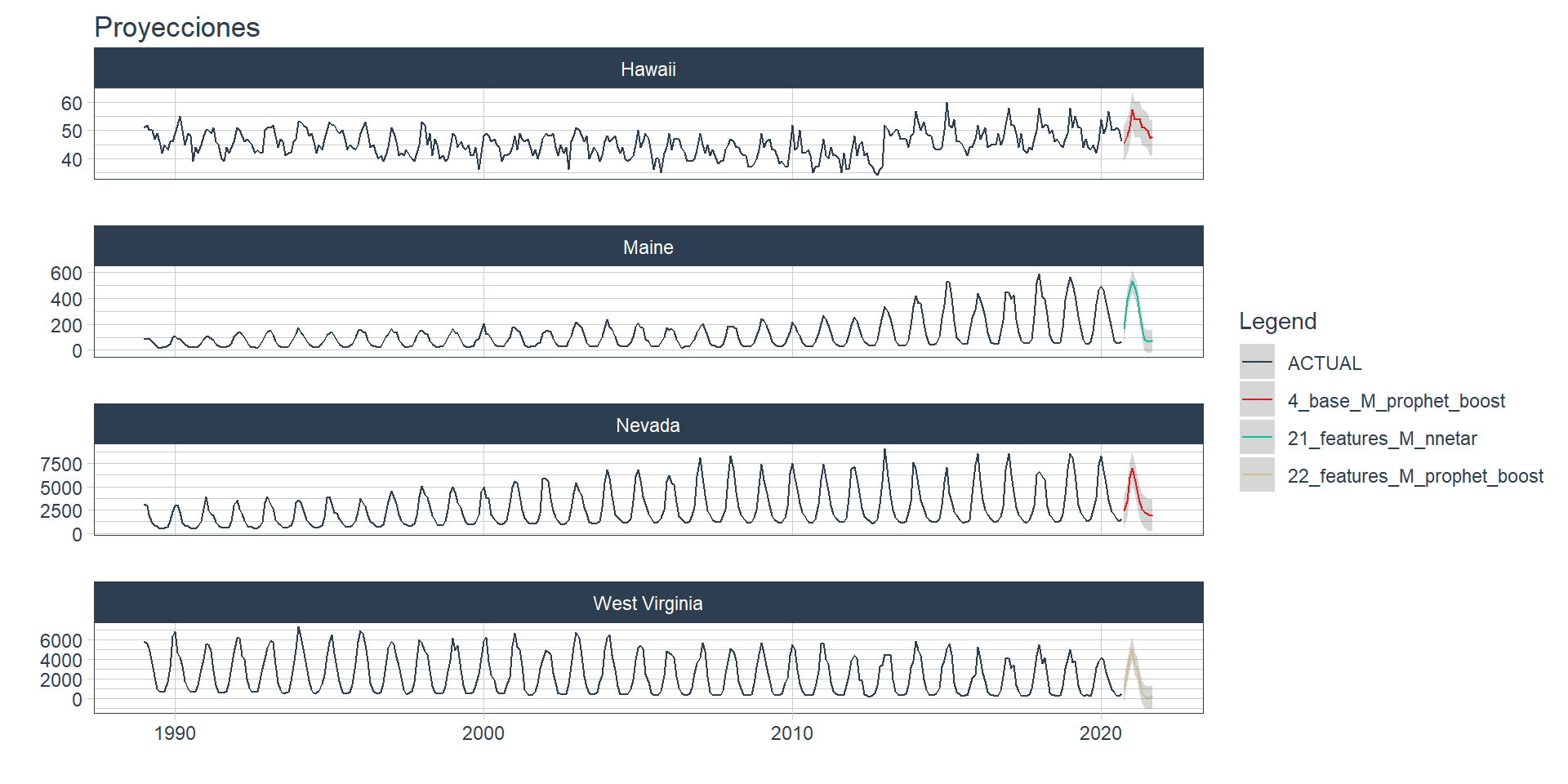
👉Time series modeling in programming languages like R or python usually takes hundreds or thousands of lines of code.
📌 In this post, we’ve explored the possibilities of using a Tidy framework (Tidymodels + Modeltime + Workflowsets) in order to better understand which model and preprocessor is better for forecasting on a specific time series.
This is an extension to out previous functions modeltiem_multi_{}, a collection of functions that expand modeltime possibilities into working with multiple time series at once.
We hope it has been useful, thanks for reading us 👏👏👏.
Karina Bartolome, Linkedin, Twitter, Github, Blogpost.
Rafael Zambrano, Linkedin, Twitter, Github, Blogpost.
For attribution, please cite this work as
Bartolomé & Zambrano (2021, April 25). Karina Bartolome: Workflowsets in Time Series. Retrieved from https://karbartolome-blog.netlify.app/posts/workflowsets-timeseries/
BibTeX citation
@misc{bartolomé2021workflowsets,
  author = {Bartolomé, Karina and Zambrano, Rafael},
  title = {Karina Bartolome: Workflowsets in Time Series},
  url = {https://karbartolome-blog.netlify.app/posts/workflowsets-timeseries/},
  year = {2021}
}